FAM-L Exam Solutions and Hints

FAM-L Exam Solutions and Hints#

actuarialmath – Solving Life Contingent Risks with Python

This package implements fundamental methods for modeling life contingent risks, and closely follows traditional topics covered in actuarial exams and standard texts such as the “Fundamentals of Actuarial Math - Long-term” exam syllabus by the Society of Actuaries, and “Actuarial Mathematics for Life Contingent Risks” by Dickson, Hardy and Waters. These code chunks demonstrate how to solve each of the sample FAM-L exam questions released by the SOA.

Sources:

SOA FAM-L Exam Questions: copy retrieved Aug 2022
SOA FAM-L Exam Solutions: copy retrieved Aug 2022
User Guide, or download pdf
API reference
Github repo and issues

# Uncomment next line to install package
# !pip install actuarialmath

"""Solutions code and hints for SOA FAM-L sample questions

MIT License.  Copyright 2022-2023, Terence Lim
"""
import math
import pandas as pd
import matplotlib.pyplot as plt
import numpy as np
from actuarialmath import Interest
from actuarialmath import Life
from actuarialmath import Survival
from actuarialmath import Lifetime
from actuarialmath import Fractional
from actuarialmath import Insurance
from actuarialmath import Annuity
from actuarialmath import Premiums
from actuarialmath import PolicyValues, Contract
from actuarialmath import Reserves
from actuarialmath import Recursion
from actuarialmath import LifeTable
from actuarialmath import SULT
from actuarialmath import SelectLife
from actuarialmath import MortalityLaws, Beta, Uniform, Makeham, Gompertz
from actuarialmath import ConstantForce
from actuarialmath import ExtraRisk
from actuarialmath import Mthly
from actuarialmath import UDD
from actuarialmath import Woolhouse

Helper to compare computed answers to expected solutions

import time
class IsClose:
    """Helper class for testing and reporting if two values are close"""
    def __init__(self, rel_tol : float = 0.01, score : bool = False,
                 verbose: bool = False):
        self.den = self.num = 0
        self.score = score      # whether to count INCORRECTs instead of assert
        self.verbose = verbose  # whether to run silently
        self.incorrect = []     # to keep list of messages for INCORRECT
        self.tol = rel_tol
        self.tic = time.time()

    def __call__(self, solution, answer, question="", rel_tol=None):
        """Compare solution to answer within relative tolerance

        Args:
          solution (str | numeric) : gold label
          answer (str | numeric) : computed answer
          question (str) : label to associate with this test
          rel_tol (float) : relative tolerance to be considered close
        """
        if isinstance(solution, str):
            isclose = (solution == answer)
        else:
            isclose = math.isclose(solution, answer, rel_tol=rel_tol or self.tol)
        self.den += 1
        self.num += isclose
        msg = f"{question} {solution}: {answer}"
        if self.verbose:
            print("-----", msg, "[OK]" if isclose else "[INCORRECT]", "-----")
        if not self.score:
            assert isclose, msg
        if not isclose:
            self.incorrect.append(msg)
        return isclose

    def __str__(self):
        """Display cumulative score and errors"""
        return f"Elapsed: {time.time()-self.tic:.1f} secs\n" \
               + f"Passed:  {self.num}/{self.den}\n" + "\n".join(self.incorrect)
isclose = IsClose(0.01, score=False, verbose=True)

1 Tables#

These tables are provided in the FAM-L exam

Interest Functions at i=0.05
Normal Distribution Table
Standard Ultimate Life Table

but you actually do not need them here!

print("Interest Functions at i=0.05")
UDD.interest_frame()

Interest Functions at i=0.05

	i(m)	d(m)	i/i(m)	d/d(m)	alpha(m)	beta(m)
1	0.05000	0.04762	1.00000	1.00000	1.00000	0.00000
2	0.04939	0.04820	1.01235	0.98795	1.00015	0.25617
4	0.04909	0.04849	1.01856	0.98196	1.00019	0.38272
12	0.04889	0.04869	1.02271	0.97798	1.00020	0.46651
0	0.04879	0.04879	1.02480	0.97600	1.00020	0.50823

print("Values of z for selected values of Pr(Z<=z)")
print(Life.quantiles_frame().to_string(float_format=lambda x: f"{x:.3f}"))

Values of z for selected values of Pr(Z<=z)
z         0.842  1.036  1.282  1.645  1.960  2.326  2.576
Pr(Z<=z)  0.800  0.850  0.900  0.950  0.975  0.990  0.995

print("Standard Ultimate Life Table at i=0.05")
SULT().frame()

Standard Ultimate Life Table at i=0.05

	l_x	q_x	a_x	A_x	2A_x	a_x:10	A_x:10	a_x:20	A_x:20	5_E_x	10_E_x	20_E_x
20	100000.0	0.000250	19.9664	0.04922	0.00580	8.0991	0.61433	13.0559	0.37829	0.78252	0.61224	0.37440
21	99975.0	0.000253	19.9197	0.05144	0.00614	8.0990	0.61433	13.0551	0.37833	0.78250	0.61220	0.37429
22	99949.7	0.000257	19.8707	0.05378	0.00652	8.0988	0.61434	13.0541	0.37837	0.78248	0.61215	0.37417
23	99924.0	0.000262	19.8193	0.05622	0.00694	8.0986	0.61435	13.0531	0.37842	0.78245	0.61210	0.37404
24	99897.8	0.000267	19.7655	0.05879	0.00739	8.0983	0.61437	13.0519	0.37848	0.78243	0.61205	0.37390
...	...	...	...	...	...	...	...	...	...	...	...	...
96	17501.8	0.192887	3.5597	0.83049	0.69991	3.5356	0.83164	3.5597	0.83049	0.19872	0.01330	0.00000
97	14125.9	0.214030	3.3300	0.84143	0.71708	3.3159	0.84210	3.3300	0.84143	0.16765	0.00827	0.00000
98	11102.5	0.237134	3.1127	0.85177	0.73356	3.1050	0.85214	3.1127	0.85177	0.13850	0.00485	0.00000
99	8469.7	0.262294	2.9079	0.86153	0.74930	2.9039	0.86172	2.9079	0.86153	0.11173	0.00266	0.00000
100	6248.2	0.289584	2.7156	0.87068	0.76427	2.7137	0.87078	2.7156	0.87068	0.08777	0.00136	0.00000

81 rows × 12 columns

2 Survival models#

SOA Question 2.1 : (B) 2.5

You are given:

$S_0(t) = \left(1 - \frac{t}{\omega} \right)^{\frac{1}{4}}, \quad 0 \le t \le \omega$
$\mu_{65} = \frac{1}{180} $

Calculate $e_{106}$, the curtate expectation of life at age 106.

hints:

derive formula for $\mu$ from given survival function
solve for $\omega$ given $\mu_{65}$
calculate $e$ by summing survival probabilities

life = Lifetime()
def mu_from_l(omega):   # first solve for omega, given mu_65 = 1/180
    return life.set_survival(l=lambda x,s: (1 - (x+s)/omega)**0.25).mu_x(65)
omega = int(life.solve(mu_from_l, target=1/180, grid=100))
e = life.set_survival(l=lambda x,s:(1 - (x + s)/omega)**.25, maxage=omega)\
        .e_x(106)       # then solve expected lifetime from omega
isclose(2.5, e, question="Q2.1")

----- Q2.1 2.5: 2.4786080555423604 [OK] -----

True

SOA Question 2.2 : (D) 400

Scientists are searching for a vaccine for a disease. You are given:

100,000 lives age x are exposed to the disease
Future lifetimes are independent, except that the vaccine, if available, will be given to all at the end of year 1
The probability that the vaccine will be available is 0.2
For each life during year 1, $q_x$ = 0.02
For each life during year 2, $q_{x+1}$ = 0.01 if the vaccine has been given and $q_{x+1}$ = 0.02 if it has not been given

Calculate the standard deviation of the number of survivors at the end of year 2.

hints:

calculate survival probabilities for the two scenarios
apply conditional variance formula (or mixed distribution)

p1 = (1. - 0.02) * (1. - 0.01)  # 2_p_x if vaccine given
p2 = (1. - 0.02) * (1. - 0.02)  # 2_p_x if vaccine not given
std = math.sqrt(Life.conditional_variance(p=.2, p1=p1, p2=p2, N=100000))
isclose(400, std, question="Q2.2")

----- Q2.2 400: 396.5914603215815 [OK] -----

True

SOA Question 2.3 : (A) 0.0483

You are given that mortality follows Gompertz Law with B = 0.00027 and c = 1.1.

Calculate $f_{50}(10)$.

hints:

Derive formula for $f$ given survival function

B, c = 0.00027, 1.1
S = lambda x,s,t: np.exp(-B * c**(x+s) * (c**t - 1)/np.log(c))
life = Survival().set_survival(S=S)
f = life.f_x(x=50, t=10)
isclose(0.0483, f, question="Q2.3")

----- Q2.3 0.0483: 0.04838918022351102 [OK] -----

True

SOA Question 2.4 : (E) 8.2

You are given $_tq_0 = \frac{t^2}{10,000} \quad 0 < t < 100$. Calculate $\overset{\circ}{e}_{75:\overline{10|}}$.

hints:

derive survival probability function $_tp_x$ given $_tq_0$
compute $\overset{\circ}{e}$ by integration

def q(t) : return (t**2)/10000. if t < 100 else 1.
e = Lifetime().set_survival(l=lambda x,s: 1 - q(x+s)).e_x(75, t=10, curtate=False)
isclose(8.2, e, question="Q2.4")

----- Q2.4 8.2: 8.20952380952381 [OK] -----

True

SOA Question 2.5 : (B) 37.1

You are given the following:

$e_{40:20} = 18$
$e_{60} = 25$
$_{20}q_{40} = 0.2$
$q_{40} = 0.003$

Calculate $e_{41}$.

hints:

solve for $e_{40}$ from limited lifetime formula
compute $e_{41}$ using forward recursion

life = Recursion(verbose=True).set_e(25, x=60, curtate=True)\
                              .set_q(0.2, x=40, t=20)\
                              .set_q(0.003, x=40)\
                              .set_e(18, x=40, t=20, curtate=True)
e = life.e_x(41, curtate=True)
isclose(37.1, e, question="Q2.5")

\[\begin{split}\begin{array}{llll} ~\texttt{Lifetime}~e_{{x+41}}~:=\\ ~~~e_{{x+41}} = [ ~e_{{x+40}} - ~e_{{x+40:\overline{1|}}} ] / ~p_{x+40}& \quad \texttt{forward recursion}\\ ~~~~~e_{{x+40}} = ~e_{{x+40:\overline{20|}}} + ~_{20}p_{x+40} * ~e_{{x+60}}& \quad \texttt{backward recursion}\\ ~~~~~~~~~_{20}p_{x+40} = 1 - ~_{{20}}q_{x+40}& \quad \texttt{complement of mortality}\\ ~~~~~~~e_{{x+40:\overline{1|}}} = ~p_{x+40}& \quad \texttt{1-year curtate shortcut}\\ ~~~~~~~~~p_{x+40} = 1 - ~q_{x+40}& \quad \texttt{complement of mortality}\end{array}\end{split}\]

----- Q2.5 37.1: 37.11434302908726 [OK] -----

True

SOA Question 2.6 : (C) 13.3

You are given the survival function:

$S_0(x) = \left( 1 − \frac{x}{60} \right)^{\frac{1}{3}}, \quad 0 \le x \le 60$

Calculate $1000 \mu_{35}$.

hints:

derive force of mortality function $\mu$ from given survival function

life = Survival().set_survival(l=lambda x,s: (1 - (x+s)/60)**(1/3))
mu = 1000 * life.mu_x(35)
isclose(13.3, mu, question="Q2.6")

----- Q2.6 13.3: 13.333333333333586 [OK] -----

True

SOA Question 2.7 : (B) 0.1477

You are given the following survival function of a newborn:

\[\begin{split} \begin{align*} S_0(x) & = 1 - \frac{x}{250}, \quad 0 \le x < 40 \\ & = 1 - \left( \frac{x}{100} \right)^2, \quad 40 \le x \le 100 \end{align*} \end{split}\]

Calculate the probability that (30) dies within the next 20 years.

hints:

calculate from given survival function

l = lambda x,s: (1-((x+s)/250) if (x+s)<40 else 1-((x+s)/100)**2)
q = Survival().set_survival(l=l).q_x(30, t=20)
isclose(0.1477, q, question="Q2.7")

----- Q2.7 0.1477: 0.1477272727272727 [OK] -----

True

SOA Question 2.8 : (C) 0.94

In a population initially consisting of 75% females and 25% males, you are given:

For a female, the force of mortality is constant and equals $\mu$
For a male, the force of mortality is constant and equals 1.5 $\mu$
At the end of 20 years, the population is expected to consist of 85% females and 15% males

Calculate the probability that a female survives one year.

hints:

relate $p_{male}$ and $p_{female}$ through the common term $\mu$ and the given proportions

def fun(mu):  # Solve first for mu, given ratio of start and end proportions
    male = Survival().set_survival(mu=lambda x,s: 1.5 * mu)
    female = Survival().set_survival(mu=lambda x,s: mu)
    return (75 * female.p_x(0, t=20)) / (25 * male.p_x(0, t=20))
mu = Survival.solve(fun, target=85/15, grid=0.5)
p = Survival().set_survival(mu=lambda x,s: mu).p_x(0, t=1)
isclose(0.94, p, question="Q2.8")

----- Q2.8 0.94: 0.9383813306903799 [OK] -----

True

3 Life tables and selection#

SOA Question 3.1 : (B) 117

You are given:

An excerpt from a select and ultimate life table with a select period of 3 years:

$x$	$\ell_{[ x ]}$	$\ell_{[x]+1}$	$\ell_{[x]+2}$	$\ell_{x+3}$	$x+3$
60	80,000	79,000	77,000	74,000	63
61	78,000	76,000	73,000	70,000	64
62	75,000	72,000	69,000	67,000	65
63	71,000	68,000	66,000	65,000	66

Deaths follow a constant force of mortality over each year of age

Calculate $1000~ _{23}q_{[60] + 0.75}$.

hints:

interpolate with constant force of maturity

life = SelectLife().set_table(l={60: [80000, 79000, 77000, 74000],
                                 61: [78000, 76000, 73000, 70000],
                                 62: [75000, 72000, 69000, 67000],
                                 63: [71000, 68000, 66000, 65000]})
q = 1000 * life.q_r(60, s=0, r=0.75, t=3, u=2)
isclose(117, q, question="Q3.1")

----- Q3.1 117: 116.7192429022082 [OK] -----

True

SOA Question 3.2 : (D) 14.7

You are given:

The following extract from a mortality table with a one-year select period:

$x$	$l_{[x]}$	$d_{[x]}$	$l_{x+1}$	$x + 1$
65	1000	40	−	66
66	955	45	−	67

Deaths are uniformly distributed over each year of age

$\overset{\circ}{e}_{[65]} = 15.0$

Calculate $\overset{\circ}{e}_{[66]}$.

hints:

UDD $\Rightarrow \overset{\circ}{e}_{x} = e_x + 0.5$
fill select table using curtate expectations

e_curtate = Fractional.e_approximate(e_complete=15)
life = SelectLife(udd=True).set_table(l={65: [1000, None,],
                                         66: [955, None]},
                                      e={65: [e_curtate, None]},
                                      d={65: [40, None,],
                                         66: [45, None]})
e = life.e_r(x=66)
isclose(14.7, e, question="Q3.2")

----- Q3.2 14.7: 14.67801047120419 [OK] -----

True

SOA Question 3.3 : (E) 1074

You are given:

An excerpt from a select and ultimate life table with a select period of 2 years:

$x$	$\ell_{[ x ]}$	$\ell_{[ x ] + 1}$	$\ell_{x + 2}$	$x + 2$
50	99,000	96,000	93,000	52
51	97,000	93,000	89,000	53
52	93,000	88,000	83,000	54
53	90,000	84,000	78,000	55

Deaths are uniformly distributed over each year of age

Calculate $10,000 ~ _{2.2}q_{[51]+0.5}$.

hints:

interpolate lives between integer ages with UDD

life = SelectLife().set_table(l={50: [99, 96, 93],
                                 51: [97, 93, 89],
                                 52: [93, 88, 83],
                                 53: [90, 84, 78]})
q = 10000 * life.q_r(51, s=0, r=0.5, t=2.2)
isclose(1074, q, question="Q3.3")

----- Q3.3 1074: 1073.684210526316 [OK] -----

True

SOA Question 3.4 : (B) 815

The SULT Club has 4000 members all age 25 with independent future lifetimes. The mortality for each member follows the Standard Ultimate Life Table.

Calculate the largest integer N, using the normal approximation, such that the probability that there are at least N survivors at age 95 is at least 90%.

hints:

compute portfolio percentile with N=4000, and mean and variance from binomial distribution

sult = SULT()
mean = sult.p_x(25, t=95-25)
var = sult.bernoulli(mean, variance=True)
pct = sult.portfolio_percentile(N=4000, mean=mean, variance=var, prob=0.1)
isclose(815, pct, question="Q3.4")

----- Q3.4 815: 815.0943255167722 [OK] -----

True

SOA Question 3.5 : (E) 106

You are given:

$x$	60	61	62	63	64	65	66	67
$l_x$	99,999	88,888	77,777	66,666	55,555	44,444	33,333	22,222

$a =~ _{3.4|2.5}q_{60}$ assuming a uniform distribution of deaths over each year of age

$b =~ _{3.4|2.5}q_{60}$ assuming a constant force of mortality over each year of age

Calculate $100,000( a − b )$

hints:

compute mortality rates by interpolating lives between integer ages, with UDD and constant force of mortality assumptions

l = [99999, 88888, 77777, 66666, 55555, 44444, 33333, 22222]
a = LifeTable(udd=True).set_table(l={age:l for age,l in zip(range(60, 68), l)})\
                       .q_r(60, u=3.4, t=2.5)
b = LifeTable(udd=False).set_table(l={age:l for age,l in zip(range(60, 68), l)})\
                        .q_r(60, u=3.4, t=2.5)
isclose(106, 100000 * (a - b), question="Q3.5")

----- Q3.5 106: 106.16575827938624 [OK] -----

True

SOA Question 3.6 : (D) 15.85

You are given the following extract from a table with a 3-year select period:

$x$	$q_{[x]}$	$q_{[x]+1}$	$q_{[x]+2}$	$q_{x+3}$	$x+3$
60	0.09	0.11	0.13	0.15	63
61	0.10	0.12	0.14	0.16	64
62	0.11	0.13	0.15	0.17	65
63	0.12	0.14	0.16	0.18	66
64	0.13	0.15	0.17	0.19	67

$e_{64} = 5.10$

Calculate $e_{[61]}$.

hints:

apply recursion formulas for curtate expectation

e = SelectLife().set_table(q={60: [.09, .11, .13, .15],
                              61: [.1, .12, .14, .16],
                              62: [.11, .13, .15, .17],
                              63: [.12, .14, .16, .18],
                              64: [.13, .15, .17, .19]},
                           e={61: [None, None, None, 5.1]})\
                .e_x(61)
isclose(5.85, e, question="Q3.6")

----- Q3.6 5.85: 5.846832 [OK] -----

True

SOA Question 3.7 : (b) 16.4

For a mortality table with a select period of two years, you are given:

$x$	$q_{[x]}$	$q_{[x]+1}$	$q_{x+2}$	$x+2$
50	0.0050	0.0063	0.0080	52
51	0.0060	0.0073	0.0090	53
52	0.0070	0.0083	0.0100	54
53	0.0080	0.0093	0.0110	55

The force of mortality is constant between integral ages.

Calculate $1000 ~_{2.5}q_{[50]+0.4}$.

hints:

use deferred mortality formula
use chain rule for survival probabilities,
interpolate between integer ages with constant force of mortality

life = SelectLife().set_table(q={50: [.0050, .0063, .0080],
                                 51: [.0060, .0073, .0090],
                                 52: [.0070, .0083, .0100],
                                 53: [.0080, .0093, .0110]})
q = 1000 * life.q_r(50, s=0, r=0.4, t=2.5)
isclose(16.4, q, question="Q3.7")

----- Q3.7 16.4: 16.420207214428586 [OK] -----

True

SOA Question 3.8 : (B) 1505

A club is established with 2000 members, 1000 of exact age 35 and 1000 of exact age 45. You are given:

Mortality follows the Standard Ultimate Life Table
Future lifetimes are independent
N is the random variable for the number of members still alive 40 years after the club is established

Using the normal approximation, without the continuity correction, calculate the smallest $n$ such that $Pr( N \ge n ) \le 0.05$.

hints:

compute portfolio means and variances from sum of 2000 independent members’ means and variances of survival.

sult = SULT()
p1 = sult.p_x(35, t=40)
p2 = sult.p_x(45, t=40)
mean = sult.bernoulli(p1) * 1000 + sult.bernoulli(p2) * 1000
var = (sult.bernoulli(p1, variance=True) * 1000
       + sult.bernoulli(p2, variance=True) * 1000)
pct = sult.portfolio_percentile(mean=mean, variance=var, prob=.95)
isclose(1505, pct, question="Q3.8")

----- Q3.8 1505: 1504.8328375406456 [OK] -----

True

SOA Question 3.9 : (E) 3850

A father-son club has 4000 members, 2000 of which are age 20 and the other 2000 are age 45. In 25 years, the members of the club intend to hold a reunion.

You are given:

All lives have independent future lifetimes.
Mortality follows the Standard Ultimate Life Table.

Using the normal approximation, without the continuity correction, calculate the 99th percentile of the number of surviving members at the time of the reunion.

hints:

compute portfolio means and variances as sum of 4000 independent members’ means and variances (of survival)
retrieve normal percentile

sult = SULT()
p1 = sult.p_x(20, t=25)
p2 = sult.p_x(45, t=25)
mean = sult.bernoulli(p1) * 2000 + sult.bernoulli(p2) * 2000
var = (sult.bernoulli(p1, variance=True) * 2000
       + sult.bernoulli(p2, variance=True) * 2000)
pct = sult.portfolio_percentile(mean=mean, variance=var, prob=.99)
isclose(3850, pct, question="Q3.9")

----- Q3.9 3850: 3850.144345130047 [OK] -----

True

SOA Question 3.10 : (C) 0.86

A group of 100 people start a Scissor Usage Support Group. The rate at which members enter and leave the group is dependent on whether they are right-handed or left-handed.

You are given the following:

The initial membership is made up of 75% left-handed members (L) and 25% right-handed members (R)
After the group initially forms, 35 new (L) and 15 new (R) join the group at the start of each subsequent year
Members leave the group only at the end of each year
$q_L$ = 0.25 for all years
$q_R$ = 0.50 for all years

Calculate the proportion of the Scissor Usage Support Group’s expected membership that is left-handed at the start of the group’s 6th year, before any new members join for that year.

hints:

reformulate the problem by reversing time: survival to year 6 is calculated in reverse as discounting by the same number of years.

interest = Interest(v=0.75)
L = 35*interest.annuity(t=4, due=False) + 75*interest.v_t(t=5)
interest = Interest(v=0.5)
R = 15*interest.annuity(t=4, due=False) + 25*interest.v_t(t=5)
isclose(0.86, L / (L + R), question="Q3.10")

----- Q3.10 0.86: 0.8578442833761983 [OK] -----

True

SOA Question 3.11 : (B) 0.03

For the country of Bienna, you are given:

Bienna publishes mortality rates in biennial form, that is, mortality rates are of the form: $_2q_{2x},$ for $x = 0,1, 2,...$
Deaths are assumed to be uniformly distributed between ages $2x$ and $2x + 2$, for $x = 0,1, 2,...$
$_2q_{50} = 0.02$
$_2q_{52} = 0.04$

Calculate the probability that (50) dies during the next 2.5 years.

hints:

calculate mortality rate by interpolating lives assuming UDD

life = LifeTable(udd=True).set_table(q={50//2: .02, 52//2: .04})
q = life.q_r(50//2, t=2.5/2)
isclose(0.03, q, question="Q3.11")

----- Q3.11 0.03: 0.0298 [OK] -----

True

SOA Question 3.12 : (C) 0.055

X and Y are both age 61. X has just purchased a whole life insurance policy. Y purchased a whole life insurance policy one year ago.

Both X and Y are subject to the following 3-year select and ultimate table:

$x$	$\ell_{[x]}$	$\ell_{[x]+1}$	$\ell_{[x] + 2}$	$\ell_{x+3}$	$x+3$
60	10,000	9,600	8,640	7,771	63
61	8,654	8,135	6,996	5,737	64
62	7,119	6,549	5,501	4,016	65
63	5,760	4,954	3,765	2,410	66

The force of mortality is constant over each year of age.

Calculate the difference in the probability of survival to age 64.5 between X and Y.

hints:

compute survival probability by interpolating lives assuming constant force

life = SelectLife(udd=False).set_table(l={60: [10000, 9600, 8640, 7771],
                                          61: [8654, 8135, 6996, 5737],
                                          62: [7119, 6549, 5501, 4016],
                                          63: [5760, 4954, 3765, 2410]})
q = life.q_r(60, s=1, t=3.5) - life.q_r(61, s=0, t=3.5)
isclose(0.055, q, question="Q3.12")

----- Q3.12 0.055: 0.05465655938591829 [OK] -----

True

SOA Question 3.13 : (B) 1.6

A life is subject to the following 3-year select and ultimate table:

$[x]$	$\ell_{[x]}$	$\ell_{[x]+1}$	$\ell_{[x]+2}$	$\ell_{x+3}$	$x+3$
55	10,000	9,493	8,533	7,664	58
56	8,547	8,028	6,889	5,630	59
57	7,011	6,443	5,395	3,904	60
58	5,853	4,846	3,548	2,210	61

You are also given:

$e_{60} = 1$
Deaths are uniformly distributed over each year of age

Calculate $\overset{\circ}{e}_{[58]+2}$ .

hints:

compute curtate expectations using recursion formulas
convert to complete expectation assuming UDD

life = SelectLife().set_table(l={55: [10000, 9493, 8533, 7664],
                                 56: [8547, 8028, 6889, 5630],
                                 57: [7011, 6443, 5395, 3904],
                                 58: [5853, 4846, 3548, 2210]},
                              e={57: [None, None, None, 1]})
e = life.e_r(x=58, s=2)
isclose(1.6, e, question="Q3.13")

----- Q3.13 1.6: 1.6003382187147688 [OK] -----

True

SOA Question 3.14 : (C) 0.345

You are given the following information from a life table:

x	$l_x$	$d_x$	$p_x$	$q_x$
95	−	−	−	0.40
96	−	−	0.20	−
97	−	72	−	1.00

You are also given:

$l_{90} = 1000$ and $l_{93} = 825$
Deaths are uniformly distributed over each year of age.

Calculate the probability that (90) dies between ages 93 and 95.5.

hints:

compute mortality by interpolating lives between integer ages assuming UDD

life = LifeTable(udd=True).set_table(l={90: 1000, 93: 825},
                                     d={97: 72},
                                     p={96: .2},
                                     q={95: .4, 97: 1})
q = life.q_r(90, u=93-90, t=95.5 - 93)
isclose(0.345, q, question="Q3.14")

----- Q3.14 0.345: 0.345 [OK] -----

True

4 Insurance benefits#

SOA Question 4.1 : (A) 0.27212

For a special whole life insurance policy issued on (40), you are given:

Death benefits are payable at the end of the year of death
The amount of benefit is 2 if death occurs within the first 20 years and is 1 thereafter
Z is the present value random variable for the payments under this insurance
i = 0.03

x	$A_x$	$_{20}E_x$
40	0.36987	0.51276
60	0.62567	0.17878

$E[Z^2] =0.24954$

Calculate the standard deviation of Z.

hints:

solve EPV as sum of term and deferred insurance
compute variance as difference of second moment and first moment squared

life = Recursion().set_interest(i=0.03)
life.set_A(0.36987, x=40).set_A(0.62567, x=60)
life.set_E(0.51276, x=40, t=20).set_E(0.17878, x=60, t=20)
Z2 = 0.24954
A = (2 * life.term_insurance(40, t=20) + life.deferred_insurance(40, u=20))
std = math.sqrt(life.insurance_variance(A2=Z2, A1=A))
isclose(0.27212, std, question="Q4.1")

----- Q4.1 0.27212: 0.2721117749374753 [OK] -----

True

SOA Question 4.2 : (D) 0.18

or a special 2-year term insurance policy on (x), you are given:

Death benefits are payable at the end of the half-year of death
The amount of the death benefit is 300,000 for the first half-year and increases by 30,000 per half-year thereafter
$q_x$ = 0.16 and $q_{x+1}$ = 0.23
$i^{(2)}$ = 0.18
Deaths are assumed to follow a constant force of mortality between integral ages
Z is the present value random variable for this insurance

Calculate Pr( Z > 277,000) .

hints:

calculate Z(t) and deferred mortality for each half-yearly t
sum the deferred mortality probabilities for periods when PV > 277000

life = LifeTable(udd=False).set_table(q={0: .16, 1: .23})\
                           .set_interest(i_m=.18, m=2)
mthly = Mthly(m=2, life=life)
Z = mthly.Z_m(0, t=2, benefit=lambda x,t: 300000 + t*30000*2)
p = Z[Z['Z'] >= 277000]['q'].sum()
isclose(0.18, p, question="Q4.2")

----- Q4.2 0.18: 0.17941813045022975 [OK] -----

True

SOA Question 4.3 : (D) 0.878

You are given:

$q_{60} = 0.01$
Using $i = 0.05, ~ A_{60:\overline{3|}} = 0.86545$
Using $i = 0.045$ calculate $A_{60:\overline{3|}}$

hints:

solve $q_{61}$ from endowment insurance EPV formula
solve $A_{60:\overline{3|}}$ with new $i=0.045$ as EPV of endowment insurance benefits.

life = Recursion(verbose=True).set_interest(i=0.05)\
                              .set_q(0.01, x=60)\
                              .set_A(0.86545, x=60, t=3, endowment=1)
q = life.q_x(x=61)
A = Recursion(verbose=True).set_interest(i=0.045)\
                           .set_q(0.01, x=60)\
                           .set_q(q, x=61)\
                           .endowment_insurance(60, t=3)
isclose(0.878, A, question="Q4.3")

\[\begin{split}\begin{array}{llll} ~\texttt{Mortality}~q_{x+61}~:=\\ ~~~q_{x+61} = ~1 - ~p_{x+61}& \quad \texttt{complement survival}\\ ~~~~~p_{x+61} = [ v - ~A_{{x+61:\overline{2|}}} ] / [v * [ 1 - ~A_{{x+62:\overline{1|}}} ]]& \quad \texttt{insurance recursion}\\ ~~~~~~~A^1_{{x+61:\overline{2|}}} = [ ~A^1_{{x+60:\overline{3|}}} / v - ~q_{x+60} * b ] / ~p_{x+60}& \quad \texttt{forward recursion}\\ ~~~~~~~~~p_{x+60} = 1 - ~q_{x+60}& \quad \texttt{complement of mortality}\end{array}\end{split}\]

\[\begin{split}\begin{array}{llll} ~\texttt{Endowment Insurance}~A_{{x+60:\overline{3|}}}~:=\\ ~~~A^1_{{x+60:\overline{3|}}} = v * [ ~q_{x+60} * b + ~p_{x+60} * ~A^1_{{x+61:\overline{2|}}} ]& \quad \texttt{backward recursion}\\ ~~~~~A^1_{{x+61:\overline{2|}}} = v * [ ~q_{x+61} * b + ~p_{x+61} * ~A^1_{{x+62:\overline{1|}}} ]& \quad \texttt{backward recursion}\\ ~~~~~~~p_{x+61} = 1 - ~q_{x+61}& \quad \texttt{complement of mortality}\\ ~~~~~~~E_{x+60} = ~p_{x+60} * v& \quad \texttt{pure endowment}\\ ~~~~~~~~~p_{x+60} = 1 - ~q_{x+60}& \quad \texttt{complement of mortality}\end{array}\end{split}\]

----- Q4.3 0.878: 0.8777667236003878 [OK] -----

True

SOA Question 4.4 : (A) 0.036

For a special increasing whole life insurance on (40), payable at the moment of death, you are given :

The death benefit at time t is $b_t = 1 + 0.2 t, \quad t \ge 0$
The interest discount factor at time t is $v(t) = (1 + 0.2 t ) − 2, \quad t \ge 0$
$_tp_{40} ~ \mu_{40+t} = 0.025~\text{if} ~ 0 \le t < 40$, otherwise $0$
Z is the present value random variable for this insurance

Calculate Var(Z).

hints:

integrate to find EPV of $Z$ and $Z^2$
variance is difference of second moment and first moment squared

x = 40
life = Insurance().set_survival(f=lambda *x: 0.025, maxage=x+40)\
                  .set_interest(v_t=lambda t: (1 + .2*t)**(-2))
def benefit(x,t): return 1 + .2 * t
A1 = life.A_x(x, benefit=benefit, discrete=False)
A2 = life.A_x(x, moment=2, benefit=benefit, discrete=False)
var = A2 - A1**2
isclose(0.036, var, question="Q4.4")

----- Q4.4 0.036: 0.03567680106032681 [OK] -----

True

SOA Question 4.5 : (C) 35200

For a 30-year term life insurance of 100,000 on (45), you are given:

The death benefit is payable at the moment of death
Mortality follows the Standard Ultimate Life Table
$\delta = 0.05$
Deaths are uniformly distributed over each year of age

Calculate the 95th percentile of the present value of benefits random variable for this insurance

hints:

interpolate between integer ages with UDD, and find lifetime that mortality rate exceeded
compute PV of death benefit paid at that time.

sult = SULT(udd=True).set_interest(delta=0.05)
Z = 100000 * sult.Z_from_prob(45, prob=0.95, discrete=False)
isclose(35200, Z, question="Q4.5")

----- Q4.5 35200: 35187.95203719652 [OK] -----

True

SOA Question 4.6 : (B) 29.85

For a 3-year term insurance of 1000 on (70), you are given:

$q^{SULT}_{70+k}$ is the mortality rate from the Standard Ultimate Life Table, for k = 0,1,2
$q_{70 + k}$ is the mortality rate used to price this insurance, for k = 0,1, 2
$q_{70 + k} = (0.95)^k q_{70+k}^{SULT}$, for k = 0,1, 2
i = 0.05

Calculate the single net premium.

hints:

calculate adjusted mortality rates
compute term insurance as EPV of benefits

sult = SULT()
life = LifeTable().set_interest(i=0.05)\
                  .set_table(q={70+k: .95**k * sult.q_x(70+k) for k in range(3)})
A = life.term_insurance(70, t=3, b=1000)
isclose(29.85, A, question="Q4.6")

----- Q4.6 29.85: 29.848351103559015 [OK] -----

True

SOA Question 4.7 : (B) 0.06

For a 25-year pure endowment of 1 on (x), you are given:

Z is the present value random variable at issue of the benefit payment
Var (Z) = 0.10 E[Z]
$_{25}p_x = 0.57$

Calculate the annual effective interest rate.

hints:

use Bernoulli shortcut formula for variance of pure endowment Z
solve for $i$, since $p$ is given.

def fun(i):
    life = Recursion(verbose=False).set_interest(i=i)\
                                   .set_p(0.57, x=0, t=25)
    return 0.1*life.E_x(0, t=25) - life.E_x(0, t=25, moment=life.VARIANCE)
i = Recursion.solve(fun, target=0, grid=[0.058, 0.066])
isclose(0.06, i, question="Q4.7")

----- Q4.7 0.06: 0.06008023738770257 [OK] -----

True

SOA Question 4.8 : (C) 191

For a whole life insurance of 1000 on (50), you are given :

The death benefit is payable at the end of the year of death
Mortality follows the Standard Ultimate Life Table
i = 0.04 in the first year, and i = 0.05 in subsequent years

Calculate the actuarial present value of this insurance.

hints:

use insurance recursion with special interest rate $i=0.04$ in first year.

def v_t(t): return 1.04**(-t) if t < 1 else 1.04**(-1) * 1.05**(-t+1)
A = SULT().set_interest(v_t=v_t).whole_life_insurance(50, b=1000)
isclose(191, A, question="Q4.8")

----- Q4.8 191: 191.12812818823548 [OK] -----

True

SOA Question 4.9 : (D) 0.5

You are given:

$A_{35:\overline{15|}} = 0.39$
$A^1_{35:\overline{15|}} = 0.25$
$A_{35} = 0.32$

Calculate $A_{50}$.

hints:

solve $_{15}E_{35}$ from endowment insurance minus term insurance
solve implicitly from whole life as term plus deferred insurance

E = Recursion().set_A(0.39, x=35, t=15, endowment=1)\
               .set_A(0.25, x=35, t=15)\
               .E_x(35, t=15)
life = Recursion(verbose=False).set_A(0.32, x=35)\
                               .set_E(E, x=35, t=15)
def fun(A): return life.set_A(A, x=50).term_insurance(35, t=15)
A = life.solve(fun, target=0.25, grid=[0.35, 0.55])
isclose(0.5, A, question="Q4.9")

\[\begin{split}\begin{array}{llll} ~\texttt{Pure Endowment}~_{15}E_{x+35}~:=\\ ~~~_{15}E_{x+35} = ~A_{{x+35:\overline{15|}}} - ~A^1_{{x+35:\overline{15|}}}& \quad \texttt{endowment insurance minus term}\end{array}\end{split}\]

----- Q4.9 0.5: 0.5 [OK] -----

True

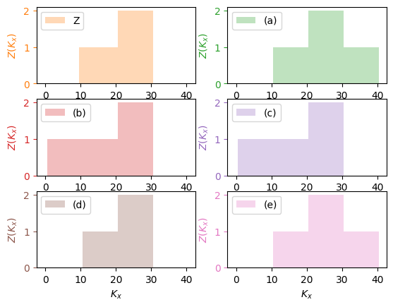
SOA Question 4.10 : (D)

The present value random variable for an insurance policy on (x) is expressed as: $$\begin{align*} Z & =0, \quad \textrm{if } T_x \le 10\\ & =v^T, \quad \textrm{if } 10 < T_x \le 20\\ & =2v^T, \quad \textrm{if } 20 < T_x \le 30\\ & =0, \quad \textrm{thereafter} \end{align*}$$

Determine which of the following is a correct expression for $E[Z]$.

(A) $_{10|}\overline{A}_x + _{20|}\overline{A}_x - _{30|}\overline{A}_x$

(B) $\overline{A}_x + _{20}E_x \overline{A}_{x+20} - 2~_{30}E_x \overline{A}_{x +30}$

(C) $_{10}E_x \overline{A}_x + _{20}E_x \overline{A}_{x+20} - 2 ~_{30}E_x \overline{A}_{x +30}$

(D) $_{10}E_x \overline{A}_{x+10} + _{20}E_x \overline{A}_{x+20} - 2~ _{30}E_x \overline{A}_{x+30}$

(E) $_{10}E_x [\overline{A}_{x} + _{10}E_{x+10} + \overline{A}_{x+20} - _{10}E_{x+20} + \overline{A}_{x+30}]$

hints:

draw and compare benefit diagrams

life = Insurance().set_interest(i=0.0).set_survival(S=lambda x,s,t: 1, maxage=40)
def fun(x, t):
    if 10 <= t <= 20: return life.interest.v_t(t)
    elif 20 < t <= 30: return 2 * life.interest.v_t(t)
    else: return 0
def A(x, t):  # Z_x+k (t-k)
    return life.interest.v_t(t - x) * (t > x)
x = 0
benefits=[lambda x,t: (life.E_x(x, t=10) * A(x+10, t)
                            + life.E_x(x, t=20)* A(x+20, t)
                            - life.E_x(x, t=30) * A(x+30, t)),
          lambda x,t: (A(x, t)
                       + life.E_x(x, t=20) * A(x+20, t)
                       - 2 * life.E_x(x, t=30) * A(x+30, t)),
          lambda x,t: (life.E_x(x, t=10) * A(x, t)
                       + life.E_x(x, t=20) * A(x+20, t)
                       - 2 * life.E_x(x, t=30) * A(x+30, t)),
          lambda x,t: (life.E_x(x, t=10) * A(x+10, t)
                       + life.E_x(x, t=20) * A(x+20, t)
                       - 2 * life.E_x(x, t=30) * A(x+30, t)),
          lambda x,t: (life.E_x(x, t=10)
                       * (A(x+10, t)
                          + life.E_x(x+10, t=10) * A(x+20, t)
                          - life.E_x(x+20, t=10) * A(x+30, t)))]
fig, ax = plt.subplots(3, 2)
ax = ax.ravel()
for i, b in enumerate([fun] + benefits):
    life.Z_plot(0, benefit=b, ax=ax[i], color=f"C{i+1}", title='')
    ax[i].legend(["(" + "abcde"[i-1] + ")" if i else "Z"])
z = [sum(abs(b(0, t) - fun(0, t)) for t in range(40)) for b in benefits]
ans = "ABCDE"[np.argmin(z)]
isclose('D', ans, question="Q4.10")

----- Q4.10 D: D [OK] -----

True

_images/f84734f2aa28fd1205b71751901a1dca44fb473e87f736d64fab273a290adafc.png

SOA Question 4.11 : (A) 143385

You are given:

$Z_1$ is the present value random variable for an n-year term insurance of 1000 issued to (x)
$Z_2$ is the present value random variable for an n-year endowment insurance of 1000 issued to (x)
For both $Z_1$ and $Z_2$ the death benefit is payable at the end of the year of death
$E [ Z_1 ] = 528$
$Var ( Z_2 ) = 15,000$
$A^{~~~~1}_{x:{\overline{n|}}} = 0.209$
$^2A^{~~~~1}_{x:{\overline{n|}}} = 0.136$

Calculate $Var(Z_1)$.

hints:

compute endowment insurance = term insurance + pure endowment
apply formula of variance as the difference of second moment and first moment squared.

A1 = 528/1000   # E[Z1]  term insurance
C1 = 0.209      # E[pure_endowment]
C2 = 0.136      # E[pure_endowment^2]
B1 = A1 + C1    # endowment = term + pure_endowment
def fun(A2):
    B2 = A2 + C2   # double force of interest
    return Insurance.insurance_variance(A2=B2, A1=B1)
A2 = Insurance.solve(fun, target=15000/(1000*1000), grid=[143400, 279300])
var = Insurance.insurance_variance(A2=A2, A1=A1, b=1000)
isclose(143385, var, question="Q4.11")

----- Q4.11 143385: 143384.99999999997 [OK] -----

True

SOA Question 4.12 : (C) 167

For three fully discrete insurance products on the same (x), you are given:

$Z_1$ is the present value random variable for a 20-year term insurance of 50
$Z_2$ is the present value random variable for a 20-year deferred whole life insurance of 100
$Z_3$ is the present value random variable for a whole life insurance of 100.
$E[Z_1] = 1.65$ and $E[Z_2] = 10.75$
$Var(Z_1) = 46.75$ and $Var(Z_2) = 50.78$

Calculate $Var(Z_3)$.

hints:

since $Z_1,~Z_2$ are non-overlapping, $E[Z_1~ Z_2] = 0$ for computing $Cov(Z_1, Z_2)$
whole life is sum of term and deferred, hence equals variance of components plus twice their covariance

cov = Life.covariance(a=1.65, b=10.75, ab=0)  # E[Z1 Z2] = 0 nonoverlapping
var = Life.variance(a=2, b=1, var_a=46.75, var_b=50.78, cov_ab=cov)
isclose(167, var, question="Q4.12")

----- Q4.12 167: 166.82999999999998 [OK] -----

True

SOA Question 4.13 : (C) 350

For a 2-year deferred, 2-year term insurance of 2000 on [65], you are given:

The following select and ultimate mortality table with a 3-year select period:

$x$	$q_{[x]}$	$q_{[x]+1}$	$q_{[x]+2}$	$q_{x+3}$	$x+3$
65	0.08	0.10	0.12	0.14	68
66	0.09	0.11	0.13	0.15	69
67	0.10	0.12	0.14	0.16	70
68	0.11	0.13	0.15	0.17	71
69	0.12	0.14	0.16	0.18	72

$i = 0.04$
The death benefit is payable at the end of the year of death

Calculate the actuarial present value of this insurance.

hints:

compute term insurance as EPV of benefits

life = SelectLife().set_table(q={65: [.08, .10, .12, .14],
                                 66: [.09, .11, .13, .15],
                                 67: [.10, .12, .14, .16],
                                 68: [.11, .13, .15, .17],
                                 69: [.12, .14, .16, .18]})\
                   .set_interest(i=.04)
A = life.deferred_insurance(65, t=2, u=2, b=2000)
isclose(350, A, question="Q4.13")

----- Q4.13 350: 351.0578236056159 [OK] -----

True

SOA Question 4.14 : (E) 390000

A fund is established for the benefit of 400 workers all age 60 with independent future lifetimes. When they reach age 85, the fund will be dissolved and distributed to the survivors.

The fund will earn interest at a rate of 5% per year.

The initial fund balance, $F$, is determined so that the probability that the fund will pay at least 5000 to each survivor is 86%, using the normal approximation.

Mortality follows the Standard Ultimate Life Table.

Calculate $F$.

hints:

discount (by interest rate $i=0.05$) the value at the portfolio percentile, of the sum of 400 bernoulli r.v. with survival probability $_{25}p_{60}$

sult = SULT()
p = sult.p_x(60, t=85-60)
mean = sult.bernoulli(p)
var = sult.bernoulli(p, variance=True)
F = sult.portfolio_percentile(mean=mean, variance=var, prob=.86, N=400)
F *= 5000 * sult.interest.v_t(85-60)
isclose(390000, F, question="Q4.14")

----- Q4.14 390000: 389322.86778416135 [OK] -----

True

SOA Question 4.15 : (E) 0.0833

For a special whole life insurance on (x), you are given :

Death benefits are payable at the moment of death
The death benefit at time $t$ is $b_t = e^{0.02t}$, for $t \ge 0$
$\mu_{x+t} = 0.04$, for $t \ge 0$
$\delta = 0.06$
Z is the present value at issue random variable for this insurance.

Calculate $Var(Z)$.

hints:

this special benefit function has effect of reducing actuarial discount rate to use in constant force of mortality shortcut formulas

life = Insurance().set_survival(mu=lambda *x: 0.04).set_interest(delta=0.06)
benefit = lambda x,t: math.exp(0.02*t)
A1 = life.A_x(0, benefit=benefit, discrete=False)
A2 = life.A_x(0, moment=2, benefit=benefit, discrete=False)
var = life.insurance_variance(A2=A2, A1=A1)
isclose(0.0833, var, question="Q4.15")

----- Q4.15 0.0833: 0.08333333333333331 [OK] -----

True

SOA Question 4.16 : (D) 0.11

You are given the following extract of ultimate mortality rates from a two-year select and ultimate mortality table:

$x$	$q_x$
50	0.045
51	0.050
52	0.055
53	0.060

The select mortality rates satisfy the following:

$q_{[x]} = 0.7 q_x$
$q_{[x]+1} = 0.8 q_{x + 1}$

You are also given that $i = 0.04$.

Calculate $A^1_{[50]:\overline{3|}}$.

hints:

compute EPV of future benefits with adjusted mortality rates

q = [.045, .050, .055, .060]
q = {50 + x: [q[x] * 0.7 if x < len(q) else None,
              q[x+1] * 0.8 if x + 1 < len(q) else None,
              q[x+2] if x + 2 < len(q) else None]
     for x in range(4)}
life = SelectLife().set_table(q=q).set_interest(i=.04)
A = life.term_insurance(50, t=3)
isclose(0.1116, A, question="Q4.16")

----- Q4.16 0.1116: 0.1115661982248521 [OK] -----

True

SOA Question 4.17 : (A) 1126.7

For a special whole life policy on (48), you are given:

The policy pays 5000 if the insured’s death is before the median curtate future lifetime at issue and 10,000 if death is after the median curtate future lifetime at issue
Mortality follows the Standard Ultimate Life Table
Death benefits are paid at the end of the year of death
i = 0.05

Calculate the actuarial present value of benefits for this policy.

hints:

find future lifetime with 50% survival probability
compute EPV of special whole life as sum of term and deferred insurance, that have different benefit amounts before and after median lifetime.

sult = SULT()
median = sult.Z_t(48, prob=0.5, discrete=False)
def benefit(x,t): return 5000 if t < median else 10000
A = sult.A_x(48, benefit=benefit)
isclose(1130, A, question="Q4.17")

----- Q4.17 1130: 1126.7747728948445 [OK] -----

True

SOA Question 4.18 : (A) 81873

You are given that T, the time to first failure of an industrial robot, has a density f(t) given by

\[\begin{split} \begin{align*} f(t) &= 0.1, \quad 0 \le t < 2\\ &= 0.4t^{-2}, \quad t \le t < 10 \end{align*} \end{split}\]

with $f(t)$ undetermined on $[10, \infty)$.

Consider a supplemental warranty on this robot that pays 100,000 at the time T of its first failure if $2 \le T \le 10$ , with no benefits payable otherwise. You are also given that $\delta = 5\%$. Calculate the 90th percentile of the present value of the future benefits under this warranty.

hints:

find values of limits such that integral of lifetime density function equals required survival probability

def f(x,s,t): return 0.1 if t < 2 else 0.4*t**(-2)
life = Insurance().set_interest(delta=0.05)\
                  .set_survival(f=f, maxage=10)
def benefit(x,t): return 0 if t < 2 else 100000
prob = 0.9 - life.q_x(0, t=2)
T = life.Z_t(0, prob=prob)
Z = life.Z_from_t(T, discrete=False) * benefit(0, T)
isclose(81873, Z, question="Q4.18")

----- Q4.18 81873: 81873.07530779815 [OK] -----

True

SOA Question 4.19 : (B) 59050

(80) purchases a whole life insurance policy of 100,000. You are given:

The policy is priced with a select period of one year
The select mortality rate equals 80% of the mortality rate from the Standard Ultimate Life Table
Ultimate mortality follows the Standard Ultimate Life Table
$i = 0.05$

Calculate the actuarial present value of the death benefits for this insurance

hints:

calculate adjusted mortality for the one-year select period
compute whole life insurance using backward recursion formula

life = SULT()
q = ExtraRisk(life=life, extra=0.8, risk="MULTIPLY_RATE")['q']
select = SelectLife(periods=1).set_select(s=0, age_selected=True, q=q)\
                              .set_select(s=1, age_selected=False, q=life['q'])\
                              .set_interest(i=.05)\
                              .fill_table()
A = 100000 * select.whole_life_insurance(80, s=0)
isclose(59050, A, question="Q4.19")

----- Q4.19 59050: 59050.59973285648 [OK] -----

True

5 Annuities#

SOA Question 5.1 : (A) 0.705

You are given:

$\delta_t = 0.06, \quad t \ge 0$
$\mu_x(t) = 0.01, \quad t \ge 0$
$Y$ is the present value random variable for a continuous annuity of 1 per year, payable for the lifetime of (x) with 10 years certain

Calculate $Pr( Y > E[Y])$.

hints:

sum annuity certain and deferred life annuity with constant force of mortality shortcut
apply equation for PV annuity r.v. Y to infer lifetime
compute survival probability from constant force of mortality function.

life = ConstantForce(mu=0.01).set_interest(delta=0.06)
EY = life.certain_life_annuity(0, u=10, discrete=False)
p = life.p_x(0, t=life.Y_to_t(EY))
isclose(0.705, p, question="Q5.1")  # 0.705

----- Q5.1 0.705: 0.7053680433746505 [OK] -----

True

SOA Question 5.2 : (B) 9.64

You are given:

$A_x = 0.30$
$A_{x + n} = 0.40$
$A^{~~~~1}_{x:\overline{n|}} = 0.35$
i = 0.05

Calculate $a_{x:\overline{n|}}$.

hints:

compute term life as difference of whole life and deferred insurance
compute twin annuity-due, and adjust to an immediate annuity.

x, n = 0, 10
a = Recursion().set_interest(i=0.05)\
               .set_A(0.3, x)\
               .set_A(0.4, x+n)\
               .set_E(0.35, x, t=n)\
               .immediate_annuity(x, t=n)
isclose(9.64, a, question="Q5.2")

\[\begin{split}\begin{array}{llll} ~\texttt{Whole Life Annuity}~\ddot{a}_{{x}}~:=\\ ~~~\ddot{a}_{{x}} = [1 - ~A_{{x}} ] / d& \quad \texttt{insurance twin}\end{array}\end{split}\]

\[\begin{split}\begin{array}{llll} ~\texttt{Whole Life Annuity}~\ddot{a}_{{x+10}}~:=\\ ~~~\ddot{a}_{{x+10}} = [1 - ~A_{{x+10}} ] / d& \quad \texttt{insurance twin}\end{array}\end{split}\]

----- Q5.2 9.64: 9.639999999999999 [OK] -----

True

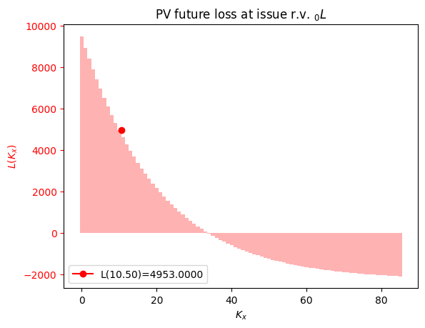
SOA Question 5.3 : (C) 6.239

You are given:

Mortality follows the Standard Ultimate Life Table
Deaths are uniformly distributed over each year of age
i = 0.05

Calculate $\frac{d}{dt}(\overline{I}\overline{a})_{40:\overline{t|}}$ at $t = 10.5$.

hints:

Differential reduces to be the EPV of the benefit payment at the upper time limit.

t = 10.5
E = t * SULT().E_r(40, t=t)
isclose(6.239, E, question="Q5.3")

----- Q5.3 6.239: 6.23871918627528 [OK] -----

True

SOA Question 5.4 : (A) 213.7

(40) wins the SOA lottery and will receive both:

A deferred life annuity of K per year, payable continuously, starting at age $40 + \overset{\circ}{e}_{40}$ and
An annuity certain of K per year, payable continuously, for $\overset{\circ}{e}_{40}$ years

You are given:

$\mu = 0.02$
$\delta = 0.01$
The actuarial present value of the payments is 10,000

Calculate K.

hints:

compute certain and life annuity factor as the sum of a certain annuity and a deferred life annuity.
solve for amount of annual benefit that equals given EPV

life = ConstantForce(mu=0.02).set_interest(delta=0.01)
u = life.e_x(40, curtate=False)
P = 10000 / life.certain_life_annuity(40, u=u, discrete=False)
isclose(213.7, P, question="Q5.4") # 213.7

----- Q5.4 213.7: 213.74552118275955 [OK] -----

True

SOA Question 5.5 : (A) 1699.6

For an annuity-due that pays 100 at the beginning of each year that (45) is alive, you are given:

Mortality for standard lives follows the Standard Ultimate Life Table
The force of mortality for standard lives age 45 + t is represented as $\mu_{45+t}^{SULT}$
The force of mortality for substandard lives age 45 + t, $\mu_{45+t}^{S}$, is defined as:

\[\begin{split}\begin{align*} \mu_{45+t}^{S} &= \mu_{45+t}^{SULT} + 0.05, \quad 0 \le t < 1\\ &= \mu_{45+t}^{SULT}, \quad t \ge 1 \end{align*}\end{split}\]

$i = 0.05$

Calculate the actuarial present value of this annuity for a substandard life age 45.

hints:

adjust mortality rate for the extra risk
compute annuity by backward recursion.

life = SULT()   # start with SULT life table
q = ExtraRisk(life=life, extra=0.05, risk="ADD_FORCE")['q']
select = SelectLife(periods=1).set_select(s=0, age_selected=True, q=q)\
                              .set_select(s=1, age_selected=False, a=life['a'])\
                              .set_interest(i=0.05)\
                              .fill_table()
a = 100 * select['a'][45][0]
isclose(1700, a, question="Q5.5")

----- Q5.5 1700: 1699.60765931901 [OK] -----

True

SOA Question 5.6 : (D) 1200

For a group of 100 lives age x with independent future lifetimes, you are given:

Each life is to be paid 1 at the beginning of each year, if alive
$A_x = 0.45$
$^2A_x = 0.22$
$i = 0.05$
$Y$ is the present value random variable of the aggregate payments.

Using the normal approximation to $Y$, calculate the initial size of the fund needed to be 95% certain of being able to make the payments for these life annuities.

hints:

compute mean and variance of EPV of whole life annuity from whole life insurance twin and variance identities.
portfolio percentile of the sum of $N=100$ life annuity payments

life = Annuity().set_interest(i=0.05)
var = life.annuity_variance(A2=0.22, A1=0.45)
mean = life.annuity_twin(A=0.45)
fund = life.portfolio_percentile(mean, var, prob=.95, N=100)
isclose(1200, fund, question="Q5.6")

----- Q5.6 1200: 1200.6946732201702 [OK] -----

True

SOA Question 5.7 : (C)

You are given:

$A_{35} = 0.188$
$A_{65} = 0.498$
$_{30}p_{35} = 0.883$
$i = 0.04$

Calculate $1000 \ddot{a}^{(2)}_{35:\overline{30|}}$ using the two-term Woolhouse approximation.

hints:

compute endowment insurance from relationships of whole life, temporary and deferred insurances.
compute temporary annuity from insurance twin
apply Woolhouse approximation

life = Recursion().set_interest(i=0.04)\
                  .set_A(0.188, x=35)\
                  .set_A(0.498, x=65)\
                  .set_p(0.883, x=35, t=30)
mthly = Woolhouse(m=2, life=life, three_term=False)
a = 1000 * mthly.temporary_annuity(35, t=30)
isclose(17376.7, a, question="Q5.7")

\[\begin{split}\begin{array}{llll} ~\texttt{Whole Life Annuity}~\ddot{a}_{{x+35}}~:=\\ ~~~\ddot{a}_{{x+35}} = [1 - ~A_{{x+35}} ] / d& \quad \texttt{insurance twin}\end{array}\end{split}\]

\[\begin{split}\begin{array}{llll} ~\texttt{Whole Life Annuity}~\ddot{a}_{{x+65}}~:=\\ ~~~\ddot{a}_{{x+65}} = [1 - ~A_{{x+65}} ] / d& \quad \texttt{insurance twin}\end{array}\end{split}\]

\[\begin{split}\begin{array}{llll} ~\texttt{Pure Endowment}~_{30}E_{x+35}~:=\\ ~~~_{30}E_{x+35} = ~_{30}p_{x+35} * v^{30}& \quad \texttt{pure endowment}\end{array}\end{split}\]

----- Q5.7 17376.7: 17376.71459632958 [OK] -----

True

SOA Question 5.8 : (C) 0.92118

For an annual whole life annuity-due of 1 with a 5-year certain period on (55), you are given:

Mortality follows the Standard Ultimate Life Table
i = 0.05

Calculate the probability that the sum of the undiscounted payments actually made under this annuity will exceed the expected present value, at issue, of the annuity.

hints:

calculate EPV of certain and life annuity.
find survival probability of lifetime s.t. sum of annual payments exceeds EPV

sult = SULT()
a = sult.certain_life_annuity(55, u=5)
p = sult.p_x(55, t=math.floor(a))
isclose(0.92118, p, question="Q5.8")

----- Q5.8 0.92118: 0.9211799771029529 [OK] -----

True

SOA Question 5.9 : (C) 0.015

hints:

express both EPV’s expressed as forward recursions
solve for unknown constant $k$.

x, p = 0, 0.9  # set arbitrary p_x = 0.9
a = Recursion().set_a(21.854, x=x)\
               .set_p(p, x=x)\
               .whole_life_annuity(x+1)
life = Recursion(verbose=False).set_a(22.167, x=x)
def fun(k): return a - life.set_p((1 + k) * p, x=x).whole_life_annuity(x + 1)
k = life.solve(fun, target=0, grid=[0.005, 0.025])
isclose(0.015, k, question="Q5.9")

\[\begin{split}\begin{array}{llll} ~\texttt{Whole Life Annuity}~\ddot{a}_{{x+1}}~:=\\ ~~~\ddot{a}_{{x+1}} = [ ~\ddot{a}_{{x}} - 1 ] / ~E_{x}& \quad \texttt{forward recursion}\\ ~~~~~~~~~E_{x} = ~p_{x} * v& \quad \texttt{pure endowment}\end{array}\end{split}\]

----- Q5.9 0.015: 0.015009110961925138 [OK] -----

True

6 Premium Calculation#

SOA Question 6.1 : (D) 35.36

6.1. You are given the following information about a special fully discrete 2-payment, 2-year term insurance on (80):

(i) Mortality follows the Standard Ultimate Life Table

(ii) i = 0.03

(iii) The death benefit is 1000 plus a return of all premiums paid without interest

(iv) Level premiums are calculated using the equivalence principle

Calculate the net premium for this special insurance.

[A modified version of Question 22 on the Fall 2012 exam]

hints:

solve net premium such that EPV annuity = EPV insurance + IA factor for returns of premiums without interest

P = SULT().set_interest(i=0.03)\
          .net_premium(80, t=2, b=1000, return_premium=True)
isclose(35.36, P, question="Q6.1")

----- Q6.1 35.36: 35.359222861900264 [OK] -----

True

SOA Question 6.2 : (E) 3604

6.2. For a fully discrete 10-year term life insurance policy on (x), you are given:

(i) Death benefits are 100,000 plus the return of all gross premiums paid without interest

(ii) Expenses are 50% of the first year’s gross premium, 5% of renewal gross premiums and 200 per policy expenses each year

(iii) Expenses are payble at the beginnig of the year

(iv) $A^1_{x:\overline{10|}} = 0.17094$

(v) $(IA)^1_{x:\overline{10|}} = 0.96728$

(vi) $\ddot{a}^1_{x:\overline{10|}} = 6.8865$

Calculate the gross premium using the equivalence principle.

[Question 25 on the Fall 2012 exam]

hints:

EPV return of premiums without interest = Premium $\times$ IA factor
solve for gross premiums such that EPV premiums = EPV benefits and expenses

life = Premiums()
A, IA, a = 0.17094, 0.96728, 6.8865
P = life.gross_premium(a=a, A=A, IA=IA, benefit=100000,
                       initial_premium=0.5, renewal_premium=.05,
                       renewal_policy=200, initial_policy=200)
isclose(3604, P, question="Q6.2")

----- Q6.2 3604: 3604.229940320728 [OK] -----

True

SOA Question 6.3 : (C) 0.390

S, now age 65, purchased a 20-year deferred whole life annuity-due of 1 per year at age 45. You are given:

Equal annual premiums, determined using the equivalence principle, were paid at the beginning of each year during the deferral period
Mortality at ages 65 and older follows the Standard Ultimate Life Table
i = 0.05
Y is the present value random variable at age 65 for S’s annuity benefits

Calculate the probability that Y is less than the actuarial accumulated value of S’s premiums.

hints:

solve lifetime $t$ such that PV annuity certain = PV whole life annuity at age 65
calculate mortality rate through the year before curtate lifetime

life = SULT()
t = life.Y_to_t(life.whole_life_annuity(65))
q = 1 - life.p_x(65, t=math.floor(t) - 1)
isclose(0.39, q, question="Q6.3")

----- Q6.3 0.39: 0.39039071872030084 [OK] -----

True

SOA Question 6.4 : (E) 1890

For whole life annuities-due of 15 per month on each of 200 lives age 62 with independent future lifetimes, you are given:

i = 0.06
$A^{12}_{62} = 0.4075$ and $^2A^{(12)}_{62} = 0.2105$
$\pi$ is the single premium to be paid by each of the 200 lives
S is the present value random variable at time 0 of total payments made to the 200 lives

Using the normal approximation, calculate $\pi$ such at $Pr(200 \pi > S) = 0.90$

mthly = Mthly(m=12, life=Annuity().set_interest(i=0.06))
A1, A2 = 0.4075, 0.2105
mean = mthly.annuity_twin(A1) * 15 * 12
var = mthly.annuity_variance(A1=A1, A2=A2, b=15 * 12)
S = Annuity.portfolio_percentile(mean=mean, variance=var, prob=.9, N=200) / 200
isclose(1890, S, question="Q6.4")

----- Q6.4 1890: 1893.912859650868 [OK] -----

True

SOA Question 6.5 : (D) 33

For a fully discrete whole life insurance of 1000 on (30), you are given:

Mortality follows the Standard Ultimate Life Table
i = 0.05
The premium is the net premium

Calculate the first year for which the expected present value at issue of that year’s premium is less than the expected present value at issue of that year’s benefit.

life = SULT()
P = life.net_premium(30, b=1000)
def gain(k):
    return life.Y_x(30, t=k) * P - life.Z_x(30, t=k) * 1000
k = min([k for k in range(100) if gain(k) < 0]) + 1  # add 1 because k=0 is first policy year
isclose(33, k, question="Q6.5")

----- Q6.5 33: 33 [OK] -----

True

SOA Question 6.6 : (B) 0.79

For fully discrete whole life insurance policies of 10,000 issued on 600 lives with independent future lifetimes, each age 62, you are given:

Mortality follows the Standard Ultimate Life Table
i = 0.05
Expenses of 5% of the first year gross premium are incurred at issue
Expenses of 5 per policy are incurred at the beginning of each policy year
The gross premium is 103% of the net premium.
$_0L$ is the aggregate present value of future loss at issue random variable

Calculate $Pr( _0L < 40,000)$, using the normal approximation.

life = SULT()
P = life.net_premium(62, b=10000)
contract = Contract(premium=1.03*P,
                    renewal_policy=5,
                    initial_policy=5,
                    initial_premium=0.05,
                    benefit=10000)
L = life.gross_policy_value(62, contract=contract)
var = life.gross_policy_variance(62, contract=contract)
prob = life.portfolio_cdf(mean=L, variance=var, value=40000, N=600)
isclose(.79, prob, question="Q6.6")

----- Q6.6 0.79: 0.7914321142683529 [OK] -----

True

SOA Question 6.7 : (C) 2880

For a special fully discrete 20-year endowment insurance on (40), you are given:

The only death benefit is the return of annual net premiums accumulated with interest at 5% to the end of the year of death
The endowment benefit is 100,000
Mortality follows the Standard Ultimate Life Table
i = 0.05

Calculate the annual net premium.

life = SULT()
a = life.temporary_annuity(40, t=20)
A = life.E_x(40, t=20)
IA = a - life.interest.annuity(t=20) * life.p_x(40, t=20)
G = life.gross_premium(a=a, A=A, IA=IA, benefit=100000)
isclose(2880, G, question="Q6.7")

----- Q6.7 2880: 2880.2463991134578 [OK] -----

True

SOA Question 6.8 : (B) 9.5

For a fully discrete whole life insurance on (60), you are given:

Mortality follows the Standard Ultimate Life Table
i = 0.05
The expected company expenses, payable at the beginning of the year, are:

50 in the first year
10 in years 2 through 10
5 in years 11 through 20
0 after year 20

Calculate the level annual amount that is actuarially equivalent to the expected company expenses.

hints:

calculate EPV of expenses as deferred life annuities
solve for level premium

life = SULT()
initial_cost = (50 + 10 * life.deferred_annuity(60, u=1, t=9)
                + 5 * life.deferred_annuity(60, u=10, t=10))
P = life.net_premium(60, initial_cost=initial_cost)
isclose(9.5, P, question="Q6.8")

----- Q6.8 9.5: 9.526003201821927 [OK] -----

True

SOA Question 6.9 : (D) 647

life = SULT()
a = life.temporary_annuity(50, t=10)
A = life.term_insurance(50, t=20)
initial_cost = 25 * life.deferred_annuity(50, u=10, t=10)
P = life.gross_premium(a=a, A=A, benefit=100000,
                       initial_premium=0.42, renewal_premium=0.12,
                       initial_policy=75 + initial_cost, renewal_policy=25)
isclose(647, P, question="Q6.9")

----- Q6.9 647: 646.8608151974504 [OK] -----

True

SOA Question 6.10 : (D) 0.91

For a fully discrete 3-year term insurance of 1000 on (x), you are given:

$p_x$ = 0.975
i = 0.06
The actuarial present value of the death benefit is 152.85
The annual net premium is 56.05

Calculate $p_{x+2}$.

x = 0
life = Recursion(depth=5).set_interest(i=0.06)\
                         .set_p(0.975, x=x)\
                         .set_a(152.85/56.05, x=x, t=3)\
                         .set_A(152.85, x=x, t=3, b=1000)
p = life.p_x(x=x+2)
isclose(0.91, p, question="Q6.10")

\[\begin{split}\begin{array}{llll} ~\texttt{Survival}~p_{x+2}~:=\\ ~~~p_{x+2} = ~E_{x+2} /v& \quad \texttt{one-year pure endowment}\\ ~~~~~E_{x+2} = ~A_{{x+2:\overline{1|}}} - ~A^1_{{x+2:\overline{1|}}}& \quad \texttt{endowment insurance minus term}\\ ~~~~~~~A^1_{{x+2:\overline{1|}}} = [ ~A^1_{{x+1:\overline{2|}}} / v - ~q_{x+1} * b ] / ~p_{x+1}& \quad \texttt{forward recursion}\\ ~~~~~~~~~p_{x+1} = [ ~\ddot{a}_{{x+1:\overline{2|}}} - 1 ] / [ v * ~\ddot{a}_{{x+2:\overline{1|}}} ]& \quad \texttt{annuity recursion}\\ ~~~~~~~~~~~\ddot{a}_{{x+1:\overline{2|}}} = [ ~\ddot{a}_{{x:\overline{3|}}} - 1 ] / ~E_{x}& \quad \texttt{forward recursion}\\ ~~~~~~~~~A^1_{{x+1:\overline{2|}}} = [ ~A^1_{{x:\overline{3|}}} / v - ~q_{x} * b ] / ~p_{x}& \quad \texttt{forward recursion}\\ ~~~~~~~~~~~~~E_{x} = ~p_{x} * v& \quad \texttt{pure endowment}\end{array}\end{split}\]

----- Q6.10 0.91: 0.9097382950525702 [OK] -----

True

SOA Question 6.11 : (C) 0.041

life = Recursion().set_interest(i=0.04)
A = life.set_A(0.39788, 51)\
        .set_q(0.0048, 50)\
        .whole_life_insurance(50)
P = life.gross_premium(A=A, a=life.annuity_twin(A=A))
A = life.set_q(0.048, 50).whole_life_insurance(50)
loss = A - life.annuity_twin(A) * P
isclose(0.041, loss, question="Q6.11")

\[\begin{split}\begin{array}{llll} ~\texttt{Whole Life Insurance}~A_{{x+50}}~:=\\ ~~~A_{{x+50}} = v * [ ~q_{x+50} * b + ~p_{x+50} * ~A_{{x+51}} ]& \quad \texttt{backward recursion}\\ ~~~~~p_{x+50} = 1 - ~q_{x+50}& \quad \texttt{complement of mortality}\end{array}\end{split}\]

----- Q6.11 0.041: 0.04069206883563675 [OK] -----

True

SOA Question 6.12 : (E) 88900

For a fully discrete whole life insurance of 1000 on (x), you are given:

The following expenses are incurred at the beginning of each year:

	Year 1	Years 2+
Percent of premium	75%	10%
Maintenance expenses	10	2

An additional expense of 20 is paid when the death benefit is paid
The gross premium is determined using the equivalence principle
$i = 0.06$
$\ddot{a}_x = 12.0$
$^2A_x = 0.14$

Calculate the variance of the loss at issue random variable.

life = PolicyValues().set_interest(i=0.06)
a = 12
A = life.insurance_twin(a)
contract = Contract(benefit=1000, settlement_policy=20,
                        initial_policy=10, initial_premium=0.75,
                        renewal_policy=2, renewal_premium=0.1)
contract.premium = life.gross_premium(A=A, a=a, **contract.premium_terms)
L = life.gross_variance_loss(A1=A, A2=0.14, contract=contract)
isclose(88900, L, question="Q6.12")

----- Q6.12 88900: 88862.59592874818 [OK] -----

True

SOA Question 6.13 : (D) -400

For a fully discrete whole life insurance of 10,000 on (45), you are given:

Commissions are 80% of the first year premium and 10% of subsequent premiums. There are no other expenses
Mortality follows the Standard Ultimate Life Table
i = 0.05
$_0L$ denotes the loss at issue random variable
If $T_{45} = 10.5$, then $_0L = 4953$

Calculate $E[_0L]$ .

life = SULT().set_interest(i=0.05)
A = life.whole_life_insurance(45)
contract = Contract(benefit=10000, initial_premium=.8, renewal_premium=.1)
def fun(P):   # Solve for premium, given Loss(t=0) = 4953
    return life.L_from_t(t=10.5, contract=contract.set_contract(premium=P))
contract.set_contract(premium=life.solve(fun, target=4953, grid=100))
L = life.gross_policy_value(45, contract=contract)
life.L_plot(x=45, T=10.5, contract=contract)
isclose(-400, L, question="Q6.13")

----- Q6.13 -400: -400.944475998793 [OK] -----

True

_images/345546dfbea126eb081671f18ecc092e694ff4b9a242915b887d69098a7765e4.png

SOA Question 6.14 : (D) 1150

For a special fully discrete whole life insurance of 100,000 on (40), you are given:

The annual net premium is P for years 1 through 10, 0.5P for years 11 through 20, and 0 thereafter
Mortality follows the Standard Ultimate Life Table
i = 0.05

Calculate P.

life = SULT().set_interest(i=0.05)
a = life.temporary_annuity(40, t=10) + 0.5*life.deferred_annuity(40, u=10, t=10)
A = life.whole_life_insurance(40)
P = life.gross_premium(a=a, A=A, benefit=100000)
isclose(1150, P, question="Q6.14")

----- Q6.14 1150: 1148.5800555155258 [OK] -----

True

SOA Question 6.15 : (B) 1.002

For a fully discrete whole life insurance of 1000 on (x) with net premiums payable quarterly, you are given:

$i = 0.05$
$\ddot{a}_x = 3.4611$
$P^{(W)}$ and $P^{(UDD)}$ are the annualized net premiums calculated using the 2-term Woolhouse (W) and the uniform distribution of deaths (UDD) assumptions, respectively

Calculate $\dfrac{P^{(UDD)}}{P^{(W)}}$.

life = Recursion().set_interest(i=0.05).set_a(3.4611, x=0)
A = life.insurance_twin(3.4611)
udd = UDD(m=4, life=life)
a1 = udd.whole_life_annuity(x=x)
woolhouse = Woolhouse(m=4, life=life)
a2 = woolhouse.whole_life_annuity(x=x)
P = life.gross_premium(a=a1, A=A)/life.gross_premium(a=a2, A=A)
isclose(1.002, P, question="Q6.15")

----- Q6.15 1.002: 1.0022973504113772 [OK] -----

True

SOA Question 6.16 : (A) 2408.6

For a fully discrete 20-year endowment insurance of 100,000 on (30), you are given:

d = 0.05
Expenses, payable at the beginning of each year, are:

	First Year	First Year	Renewal Years	Renewal Years
	Percent of Premium	Per Policy	Percent of Premium	Per Policy
Taxes	4%	0	4%	0
Sales Commission	35%	0	2%	0
Policy Maintenance	0%	250	0%	50

The net premium is 2143

Calculate the gross premium using the equivalence principle.

life = Premiums().set_interest(d=0.05)
A = life.insurance_equivalence(premium=2143, b=100000)
a = life.annuity_equivalence(premium=2143, b=100000)
p = life.gross_premium(A=A, a=a, benefit=100000, settlement_policy=0,
                       initial_policy=250, initial_premium=0.04 + 0.35,
                       renewal_policy=50, renewal_premium=0.04 + 0.02)
isclose(2410, p, question="Q6.16")

----- Q6.16 2410: 2408.575206281868 [OK] -----

True

SOA Question 6.17 : (A) -30000

An insurance company sells special fully discrete two-year endowment insurance policies to smokers (S) and non-smokers (NS) age x. You are given:

The death benefit is 100,000; the maturity benefit is 30,000
The level annual premium for non-smoker policies is determined by the equivalence principle
The annual premium for smoker policies is twice the non-smoker annual premium
$\mu^{NS}_{x+t} = 0.1.\quad t > 0$
$q^S_{x+k} = 1.5 q_{x+k}^{NS}$, for $k = 0, 1$
$i = 0.08$

Calculate the expected present value of the loss at issue random variable on a smoker policy.

x = 0
life = ConstantForce(mu=0.1).set_interest(i=0.08)
A = life.endowment_insurance(x, t=2, b=100000, endowment=30000)
a = life.temporary_annuity(x, t=2)
P = life.gross_premium(a=a, A=A)
life1 = Recursion().set_interest(i=0.08)\
                   .set_q(life.q_x(x, t=1) * 1.5, x=x, t=1)\
                   .set_q(life.q_x(x+1, t=1) * 1.5, x=x+1, t=1)
contract = Contract(premium=P*2, benefit=100000, endowment=30000)
L = life1.gross_policy_value(x, t=0, n=2, contract=contract)
isclose(-30000, L, question="Q6.17")

\[\begin{split}\begin{array}{llll} ~\texttt{Term Insurance}~A^1_{{x:\overline{2|}}}~:=\\ ~~~A^1_{{x:\overline{2|}}} = ~A_{{x:\overline{2|}}} - ~_{2}E_{x}& \quad \texttt{endowment insurance - pure}\\ ~~~~~_{2}E_{x} = ~_{2}p_{x} * v^{2}& \quad \texttt{pure endowment}\\ ~~~~~~~_{2}p_{x} = ~p_{x+1} * ~p_{x}& \quad \texttt{survival chain rule}\\ ~~~~~A^1_{{x:\overline{2|}}} = v * [ ~q_{x} * b + ~p_{x} * ~A^1_{{x+1:\overline{1|}}} ]& \quad \texttt{backward recursion}\\ ~~~~~~~p_{x+1} = 1 - ~q_{x+1}& \quad \texttt{complement of mortality}\\ ~~~~~~~~~E_{x} = ~p_{x} * v& \quad \texttt{pure endowment}\\ ~~~~~~~~~p_{x} = 1 - ~q_{x}& \quad \texttt{complement of mortality}\end{array}\end{split}\]

\[\begin{split}\begin{array}{llll} ~\texttt{Temporary Annuity}~\ddot{a}_{{x:\overline{2|}}}~:=\\ ~~~\ddot{a}_{{x:\overline{2|}}} = 1 + ~E_{x} * ~\ddot{a}_{{x+1:\overline{1|}}}& \quad \texttt{backward recursion}\\ ~~~~~E_{x} = ~p_{x} * v& \quad \texttt{pure endowment}\\ ~~~~~~~p_{x} = 1 - ~q_{x}& \quad \texttt{complement of mortality}\end{array}\end{split}\]

\[\begin{split}\begin{array}{llll} ~\texttt{Pure Endowment}~_{2}E_{x}~:=\\ ~~~_{2}E_{x} = ~_{2}p_{x} * v^{2}& \quad \texttt{pure endowment}\\ ~~~~~_{2}p_{x} = ~p_{x+1} * ~p_{x}& \quad \texttt{survival chain rule}\\ ~~~~~~~p_{x} = 1 - ~q_{x}& \quad \texttt{complement of mortality}\\ ~~~~~~~~~p_{x+1} = 1 - ~q_{x+1}& \quad \texttt{complement of mortality}\end{array}\end{split}\]

----- Q6.17 -30000: -30107.42633581128 [OK] -----

True

SOA Question 6.18 : (D) 166400

For a 20-year deferred whole life annuity-due with annual payments of 30,000 on (40), you are given:

The single net premium is refunded without interest at the end of the year of death if death occurs during the deferral period
Mortality follows the Standard Ultimate Life Table
i = 0.05

Calculate the single net premium for this annuity.

life = SULT().set_interest(i=0.05)
def fun(P):
    A = (life.term_insurance(40, t=20, b=P)
         + life.deferred_annuity(40, u=20, b=30000))
    return life.gross_premium(a=1, A=A) - P
P = life.solve(fun, target=0, grid=[162000, 168800])
isclose(166400, P, question="Q6.18")

----- Q6.18 166400: 166362.83871487685 [OK] -----

True

SOA Question 6.19 : (B) 0.033

life = SULT()
contract = Contract(initial_policy=.2, renewal_policy=.01)
a = life.whole_life_annuity(50)
A = life.whole_life_insurance(50)
contract.premium = life.gross_premium(A=A, a=a, **contract.premium_terms)
L = life.gross_policy_variance(50, contract=contract)
isclose(0.033, L, question="Q6.19")

----- Q6.19 0.033: 0.03283273381910881 [OK] -----

True

SOA Question 6.20 : (B) 459

For a special fully discrete 3-year term insurance on (75), you are given:

The death benefit during the first two years is the sum of the net premiums paid without interest
The death benefit in the third year is 10,000

$x$	$p_x$
75	0.90
76	0.88
77	0.85

$i = 0.04$

Calculate the annual net premium.

life = LifeTable().set_interest(i=.04).set_table(p={75: .9, 76: .88, 77: .85})
a = life.temporary_annuity(75, t=3)
IA = life.increasing_insurance(75, t=2)
A = life.deferred_insurance(75, u=2, t=1)
def fun(P): return life.gross_premium(a=a, A=P*IA + A*10000) - P
P = life.solve(fun, target=0, grid=[449, 489])
isclose(459, P, question="Q6.20")

----- Q6.20 459: 458.83181728297365 [OK] -----

True

SOA Question 6.21 : (C) 100

life = Recursion(verbose=False).set_interest(d=0.04)
life.set_A(0.7, x=75, t=15, endowment=1)
life.set_E(0.11, x=75, t=15)
def fun(P):
    return (P * life.temporary_annuity(75, t=15) -
            life.endowment_insurance(75, t=15, b=1000, endowment=15*float(P)))
P = life.solve(fun, target=0, grid=(80, 120))
isclose(100, P, question="Q6.21")

----- Q6.21 100: 100.85470085470084 [OK] -----

/tmp/ipykernel_20933/899435277.py:6: DeprecationWarning: Conversion of an array with ndim > 0 to a scalar is deprecated, and will error in future. Ensure you extract a single element from your array before performing this operation. (Deprecated NumPy 1.25.)
  life.endowment_insurance(75, t=15, b=1000, endowment=15*float(P)))

True

SOA Question 6.22 : (C) 102

For a whole life insurance of 100,000 on (45) with premiums payable monthly for a period of 20 years, you are given:

The death benefit is paid immediately upon death
Mortality follows the Standard Ultimate Life Table
Deaths are uniformly distributed over each year of age
$i = 0.05$

Calculate the monthly net premium.

life=SULT(udd=True)
a = UDD(m=12, life=life).temporary_annuity(45, t=20)
A = UDD(m=0, life=life).whole_life_insurance(45)
P = life.gross_premium(A=A, a=a, benefit=100000) / 12
isclose(102, P, question="Q6.22")

----- Q6.22 102: 102.40668704849178 [OK] -----

True

SOA Question 6.23 : (D) 44.7

x = 0
life = Recursion().set_a(15.3926, x=x)\
                  .set_a(10.1329, x=x, t=15)\
                  .set_a(14.0145, x=x, t=30)
def fun(P):
    per_policy = 30 + (30 * life.whole_life_annuity(x))
    per_premium = (0.6 + 0.1*life.temporary_annuity(x, t=15)
                    + 0.1*life.temporary_annuity(x, t=30))
    a = life.temporary_annuity(x, t=30)
    return (P * a) - (per_policy + per_premium * P)
P = life.solve(fun, target=0, grid=[30.3, 49.5])
isclose(44.7, P, question="Q6.23")

----- Q6.23 44.7: 44.70806635781145 [OK] -----

True

SOA Question 6.24 : (E) 0.30

For a fully continuous whole life insurance of 1 on (x), you are given:

L is the present value of the loss at issue random variable if the premium rate is determined by the equivalence principle
L^* is the present value of the loss at issue random variable if the premium rate is 0.06
$\delta = 0.07$
$\overline{A}_x = 0.30$
$Var(L) = 0.18$

Calculate $Var(L^*)$.

life = PolicyValues().set_interest(delta=0.07)
x, A1 = 0, 0.30   # Policy for first insurance
P = life.premium_equivalence(A=A1, discrete=False)  # Need its premium
contract = Contract(premium=P, discrete=False)
def fun(A2):  # Solve for A2, given Var(Loss)
    return life.gross_variance_loss(A1=A1, A2=A2, contract=contract)
A2 = life.solve(fun, target=0.18, grid=0.18)

contract = Contract(premium=0.06, discrete=False) # Solve second insurance
var = life.gross_variance_loss(A1=A1, A2=A2, contract=contract)
isclose(0.304, var, question="Q6.24")

----- Q6.24 0.304: 0.30419999999999975 [OK] -----

True

SOA Question 6.25 : (C) 12330

For a fully discrete 10-year deferred whole life annuity-due of 1000 per month on (55), you are given:

The premium, $G$, will be paid annually at the beginning of each year during the deferral period
Expenses are expected to be 300 per year for all years, payable at the beginning of the year
Mortality follows the Standard Ultimate Life Table
$i = 0.05$
Using the two-term Woolhouse approximation, the expected loss at issue is -800

Calculate $G$.

life = SULT()
woolhouse = Woolhouse(m=12, life=life)
benefits = woolhouse.deferred_annuity(55, u=10, b=1000 * 12)
expenses = life.whole_life_annuity(55, b=300)
payments = life.temporary_annuity(55, t=10)
def fun(P):
    return life.gross_future_loss(A=benefits + expenses, a=payments,
                                  contract=Contract(premium=P))
P = life.solve(fun, target=-800, grid=[12110, 12550])
isclose(12330, P, question="Q6.25")

----- Q6.25 12330: 12325.781125438532 [OK] -----

True

SOA Question 6.26 : (D) 180

For a special fully discrete whole life insurance policy of 1000 on (90), you are given:

The first year premium is 0
P is the renewal premium
Mortality follows the Standard Ultimate Life Table
i = 0.05
Premiums are calculated using the equivalence principle

Calculate P.

life = SULT().set_interest(i=0.05)
def fun(P):
    return P - life.net_premium(90, b=1000, initial_cost=P)
P = life.solve(fun, target=0, grid=[150, 190])
isclose(180, P, question="Q6.26")

----- Q6.26 180: 180.03164891315893 [OK] -----

True

SOA Question 6.27 : (D) 10310

For a special fully continuous whole life insurance on (x), you are given:

Premiums and benefits:

	First 20 years	After 20 years
Premium Rate	3P	P
Benefit	1,000,000	500,000

$\mu_{x+t} = 0.03, \quad t \ge 0$
$\delta = 0.06$

Calculate $P$ using the equivalence principle.

life = ConstantForce(mu=0.03).set_interest(delta=0.06)
x = 0
payments = (3 * life.temporary_annuity(x, t=20, discrete=False)
            + life.deferred_annuity(x, u=20, discrete=False))
benefits = (1000000 * life.term_insurance(x, t=20, discrete=False)
            + 500000 * life.deferred_insurance(x, u=20, discrete=False))
P = benefits / payments
isclose(10310, P, question="Q6.27")

----- Q6.27 10310: 10309.617799001708 [OK] -----

True

SOA Question 6.28 : (B) 36

life = SULT().set_interest(i=0.05)
a = life.temporary_annuity(40, t=5)
A = life.whole_life_insurance(40)
P = life.gross_premium(a=a, A=A, benefit=1000,
                       initial_policy=10, renewal_premium=.05,
                       renewal_policy=5, initial_premium=.2)
isclose(36, P, question="Q6.28")

----- Q6.28 36: 35.72634219391481 [OK] -----

True

SOA Question 6.29 : (B) 20.5

(35) purchases a fully discrete whole life insurance policy of 100,000. You are given:

The annual gross premium, calculated using the equivalence principle, is 1770
The expenses in policy year 1 are 50% of premium and 200 per policy
The expenses in policy years 2 and later are 10% of premium and 50 per policy
All expenses are incurred at the beginning of the policy year
$i = 0.035$

Calculate $\ddot{a}_{35}$.

life = Premiums().set_interest(i=0.035)
def fun(a):
    return life.gross_premium(A=life.insurance_twin(a=a), a=a,
                              initial_policy=200, initial_premium=.5,
                              renewal_policy=50, renewal_premium=.1,
                              benefit=100000)
a = life.solve(fun, target=1770, grid=[20, 22])
isclose(20.5, a, question="Q6.29")

----- Q6.29 20.5: 20.480268314431726 [OK] -----

True

SOA Question 6.30 : (A) 900

For a fully discrete whole life insurance of 100 on (x), you are given:

The first year expense is 10% of the gross annual premium
Expenses in subsequent years are 5% of the gross annual premium
The gross premium calculated using the equivalence principle is 2.338
$i = 0.04$
$\ddot{a}_x = 16.50$
$^2A_x = 0.17$

Calculate the variance of the loss at issue random variable.

life = PolicyValues().set_interest(i=0.04)
contract = Contract(premium=2.338,
                    benefit=100,
                    initial_premium=.1,
                    renewal_premium=0.05)
var = life.gross_variance_loss(A1=life.insurance_twin(16.50),
                               A2=0.17, contract=contract)
isclose(900, var, question="Q6.30")

----- Q6.30 900: 908.141412994607 [OK] -----

True

SOA Question 6.31 : (D) 1330

For a fully continuous whole life insurance policy of 100,000 on (35), you are given:

The density function of the future lifetime of a newborn: $$\begin{align*} f(t) & = 0.01 e^{-0.01 t}, \quad 0 \le t < 70\\ & = g(t), \quad t \ge 70 \end{align*}$$
$\delta = 0.05$
$\overline{A}_{70} = 0.51791$

Calculate the annual net premium rate for this policy.

life = ConstantForce(mu=0.01).set_interest(delta=0.05)
A = (life.term_insurance(35, t=35, discrete=False)
     + life.E_x(35, t=35)*0.51791)     # A_35
P = life.premium_equivalence(A=A, b=100000, discrete=False)
isclose(1330, P, question="Q6.31")

----- Q6.31 1330: 1326.5406293909457 [OK] -----

True

SOA Question 6.32 : (C) 550

For a whole life insurance of 100,000 on (x), you are given:

Death benefits are payable at the moment of death
Deaths are uniformly distributed over each year of age
Premiums are payable monthly
$i = 0.05$
$\ddot{a}_x = 9.19$

Calculate the monthly net premium.

x = 0
life = Recursion().set_interest(i=0.05).set_a(9.19, x=x)
benefits = UDD(m=0, life=life).whole_life_insurance(x)
payments = UDD(m=12, life=life).whole_life_annuity(x)
P = life.gross_premium(a=payments, A=benefits, benefit=100000)/12
isclose(550, P, question="Q6.32")

\[\begin{split}\begin{array}{llll} ~\texttt{Whole Life Insurance}~A_{{x}}~:=\\ ~~~\ddot{a}_{{x}} = [ 1 - ~A_{{x}} ] / d& \quad \texttt{annuity twin}\end{array}\end{split}\]

----- Q6.32 550: 550.4356936711871 [OK] -----

True

SOA Question 6.33 : (B) 0.13

An insurance company sells 15-year pure endowments of 10,000 to 500 lives, each age x, with independent future lifetimes. The single premium for each pure endowment is determined by the equivalence principle.

You are given:

$i$ = 0.03
$\mu_x(t) = 0.02 t, \quad t \ge 0$
$_0L$ is the aggregate loss at issue random variable for these pure endowments.

Using the normal approximation without continuity correction, calculate $Pr(_0L) > 50,000)$.

life = Insurance().set_survival(mu=lambda x,t: 0.02*t).set_interest(i=0.03)
x = 0
var = life.E_x(x, t=15, moment=life.VARIANCE, endowment=10000)
p = 1- life.portfolio_cdf(mean=0, variance=var, value=50000, N=500)
isclose(0.13, p, question="Q6.33", rel_tol=0.02)

----- Q6.33 0.13: 0.12828940905648634 [OK] -----

True

SOA Question 6.34 : (A) 23300

For a fully discrete whole life insurance policy on (61), you are given:

The annual gross premium using the equivalence principle is 500
Initial expenses, incurred at policy issue, are 15% of the premium
Renewal expenses, incurred at the beginning of each year after the first, are 3% of the premium
Mortality follows the Standard Ultimate Life Table
i = 0.05

Calculate the amount of the death benefit.

life = SULT()
def fun(benefit):
    A = life.whole_life_insurance(61)
    a = life.whole_life_annuity(61)
    return life.gross_premium(A=A, a=a, benefit=benefit,
                              initial_premium=0.15, renewal_premium=0.03)
b = life.solve(fun, target=500, grid=[23300, 23700])
isclose(23300, b, question="Q6.34")

----- Q6.34 23300: 23294.288659265632 [OK] -----

True

SOA Question 6.35 : (D) 530

For a fully discrete whole life insurance policy of 100,000 on (35), you are given:

First year commissions are 19% of the annual gross premium
Renewal year commissions are 4% of the annual gross premium
Mortality follows the Standard Ultimate Life Table
$i = 0.05$

Calculate the annual gross premium for this policy using the equivalence principle.

sult = SULT()
A = sult.whole_life_insurance(35, b=100000)
a = sult.whole_life_annuity(35)
P = sult.gross_premium(a=a, A=A, initial_premium=.19, renewal_premium=.04)
isclose(530, P, question="Q6.35")

----- Q6.35 530: 534.4072234303343 [OK] -----

True

SOA Question 6.36 : (B) 500

life = ConstantForce(mu=0.04).set_interest(delta=0.08)
a = life.temporary_annuity(50, t=20, discrete=False)
A = life.term_insurance(50, t=20, discrete=False)
def fun(R):
    return life.gross_premium(a=a, A=A, initial_premium=R/4500,
                              renewal_premium=R/4500, benefit=100000)
R = life.solve(fun, target=4500, grid=[400, 800])
isclose(500, R, question="Q6.36")

----- Q6.36 500: 500.0 [OK] -----

True

SOA Question 6.37 : (D) 820

For a fully discrete whole life insurance policy of 50,000 on (35), with premiums payable for a maximum of 10 years, you are given:

Expenses of 100 are payable at the end of each year including the year of death
Mortality follows the Standard Ultimate Life Table
$i = 0.05$

Calculate the annual gross premium using the equivalence principle.

sult = SULT()
benefits = sult.whole_life_insurance(35, b=50000 + 100)
expenses = sult.immediate_annuity(35, b=100)
a = sult.temporary_annuity(35, t=10)
P = (benefits + expenses) / a
isclose(820, P, question="Q6.37")

----- Q6.37 820: 819.7190338249138 [OK] -----

True

SOA Question 6.38 : (B) 11.3

For an n-year endowment insurance of 1000 on (x), you are given:

Death benefits are payable at the moment of death
Premiums are payable annually at the beginning of each year
Deaths are uniformly distributed over each year of age
$i = 0.05$
$_nE_x = 0.172$
$\overline{A}_{x:\overline{n|}} = 0.192$

Calculate the annual net premium for this insurance.

x, n = 0, 10
life = Recursion().set_interest(i=0.05)\
                  .set_A(0.192, x=x, t=n, endowment=1, discrete=False)\
                  .set_E(0.172, x=x, t=n)
a = life.temporary_annuity(x, t=n, discrete=False)

def fun(a):   # solve for discrete annuity, given continuous
    life = Recursion(verbose=False).set_interest(i=0.05)\
                                   .set_a(a, x=x, t=n)\
                                   .set_E(0.172, x=x, t=n)
    return UDD(m=0, life=life).temporary_annuity(x, t=n)
a = life.solve(fun, target=a, grid=a)  # discrete annuity
P = life.gross_premium(a=a, A=0.192, benefit=1000)
isclose(11.3, P, question="Q6.38")

\[\begin{split}\begin{array}{llll} ~\texttt{Temporary Annuity}~a_{{x:\overline{10|}}}~:=\\ ~~~\ddot{a}_{{x:\overline{10|}}} = [ 1 - ~A_{{x:\overline{10|}}} ] / d& \quad \texttt{annuity twin}\end{array}\end{split}\]

----- Q6.38 11.3: 11.308644185253657 [OK] -----

True

SOA Question 6.39 : (A) 29

XYZ Insurance writes 10,000 fully discrete whole life insurance policies of 1000 on lives age 40 and an additional 10,000 fully discrete whole life policies of 1000 on lives age 80.

XYZ used the following assumptions to determine the net premiums for these policies:

Mortality follows the Standard Ultimate Life Table
i = 0.05

During the first ten years, mortality did follow the Standard Ultimate Life Table.

Calculate the average net premium per policy in force received at the beginning of the eleventh year.

sult = SULT()
P40 = sult.premium_equivalence(sult.whole_life_insurance(40), b=1000)
P80 = sult.premium_equivalence(sult.whole_life_insurance(80), b=1000)
p40 = sult.p_x(40, t=10)
p80 = sult.p_x(80, t=10)
P = (P40 * p40 + P80 * p80) / (p80 + p40)
isclose(29, P, question="Q6.39")

----- Q6.39 29: 29.03386642784549 [OK] -----

True

SOA Question 6.40 : (C) 116

For a special fully discrete whole life insurance, you are given:

The death benefit is $1000(1.03)^k$ for death in policy year k, for $k = 1, 2, 3...$
$q_x = 0.05$
$i = 0.06$
$\ddot{a}_{x+1} = 7.00$
The annual net premium for this insurance at issue age x is 110

Calculate the annual net premium for this insurance at issue age $x + 1$.

# - standard formula discounts/accumulates by too much (i should be smaller)
x = 0
life = Recursion().set_interest(i=0.06).set_a(7, x=x+1).set_q(0.05, x=x)
a = life.whole_life_annuity(x)
A = 110 * a / 1000
life = Recursion().set_interest(i=0.06).set_A(A, x=x).set_q(0.05, x=x)
A1 = life.whole_life_insurance(x+1)
P = life.gross_premium(A=A1 / 1.03, a=7) * 1000
isclose(116, P, question="Q6.40")

\[\begin{split}\begin{array}{llll} ~\texttt{Whole Life Annuity}~\ddot{a}_{{x}}~:=\\ ~~~\ddot{a}_{{x}} = 1 + ~E_{x} * ~\ddot{a}_{{x+1}}& \quad \texttt{backward recursion}\\ ~~~~~E_{x} = ~p_{x} * v& \quad \texttt{pure endowment}\\ ~~~~~~~p_{x} = 1 - ~q_{x}& \quad \texttt{complement of mortality}\end{array}\end{split}\]

\[\begin{split}\begin{array}{llll} ~\texttt{Whole Life Insurance}~A_{{x+1}}~:=\\ ~~~A_{{x+1}} = [ ~A_{{x}} / v - ~q_{x} * b ] / ~p_{x}& \quad \texttt{forward recursion}\\ ~~~~~~~~~p_{x} = 1 - ~q_{x}& \quad \texttt{complement of mortality}\end{array}\end{split}\]

----- Q6.40 116: 116.51945397474269 [OK] -----

True

SOA Question 6.41 : (B) 1417

For a special fully discrete 2-year term insurance on (x), you are given:

$q_x = 0.01$
$q_{x + 1} = 0.02$
$i = 0.05$
The death benefit in the first year is 100,000
Both the benefits and premiums increase by 1% in the second year

Calculate the annual net premium in the first year.

x = 0
life = LifeTable().set_interest(i=0.05).set_table(q={x:.01, x+1:.02})
a = 1 + life.E_x(x, t=1) * 1.01
A = life.deferred_insurance(x, u=0, t=1) + 1.01*life.deferred_insurance(x, u=1, t=1)
P = 100000 * A / a
isclose(1417, P, question="Q6.41")

----- Q6.41 1417: 1416.9332301924137 [OK] -----

True

SOA Question 6.42 : (D) 0.113

x = 0
life = ConstantForce(mu=0.06).set_interest(delta=0.06)
contract = Contract(discrete=True, premium=315.8,
                    T=3, endowment=1000, benefit=1000)
L = [life.L_from_t(t, contract=contract) for t in range(3)]    # L(t)
Q = [life.q_x(x, u=u, t=1) for u in range(3)]              # prob(die in year t)
Q[-1] = 1 - sum(Q[:-1])   # follows SOA Solution: incorrectly treats endowment!
p = sum([q for (q, l) in zip (Q, L) if l > 0])
isclose(0.113, p, question="Q6.42")

----- Q6.42 0.113: 0.11307956328284252 [OK] -----

True

SOA Question 6.43 : (C) 170

For a fully discrete, 5-payment 10-year term insurance of 200,000 on (30), you are given:

Mortality follows the Standard Ultimate Life Table
The following expenses are incurred at the beginning of each respective year:

	Percent of Premium	Per Policy	Percent of Premium	Per Policy
	Year 1	Year 1	Years 2 - 10	Years 2 - 10
Taxes	5%	0	5%	0
Commissions	30%	0	10%	0
Maintenance	0%	8	0%	4

i = 0.05
$\ddot{a}_{30:\overline{5|}} = 4.5431$

Calculate the annual gross premium using the equivalence principle.

although 10-year term, premiums only paid first first years: separately calculate the EPV of per-policy maintenance expenses in years 6-10 and treat as additional initial expense

sult = SULT()
a = sult.temporary_annuity(30, t=5)
A = sult.term_insurance(30, t=10)
other_expenses = 4 * sult.deferred_annuity(30, u=5, t=5)
P = sult.gross_premium(a=a, A=A, benefit=200000, initial_premium=0.35,
                       initial_policy=8 + other_expenses, renewal_policy=4,
                       renewal_premium=0.15)
isclose(170, P, question="Q6.43")

----- Q6.43 170: 171.22371939459944 [OK] -----

True

SOA Question 6.44 : (D) 2.18

life = Recursion().set_interest(i=0.05)\
                  .set_IA(0.15, x=50, t=10)\
                  .set_a(17, x=50)\
                  .set_a(15, x=60)\
                  .set_E(0.6, x=50, t=10)
A = life.deferred_insurance(50, u=10)
IA = life.increasing_insurance(50, t=10)
a = life.temporary_annuity(50, t=10)
P = life.gross_premium(a=a, A=A, IA=IA, benefit=100)
isclose(2.2, P, question="Q6.44")

\[\begin{split}\begin{array}{llll} ~\texttt{Whole Life Insurance}~A_{{x+60}}~:=\\ ~~~\ddot{a}_{{x+60}} = [ 1 - ~A_{{x+60}} ] / d& \quad \texttt{annuity twin}\end{array}\end{split}\]

----- Q6.44 2.2: 2.183803457688809 [OK] -----

True

SOA Question 6.45 : (E) 690

For a fully continuous whole life insurance of 100,000 on (35), you are given:

The annual rate of premium is 560
Mortality follows the Standard Ultimate Life Table
Deaths are uniformly distributed over each year of age
i = 0.05

Calculate the 75th percentile of the loss at issue random variable for this policy.

life = SULT(udd=True)
contract = Contract(benefit=100000, premium=560, discrete=False)
L = life.L_from_prob(x=35, prob=0.75, contract=contract)
life.L_plot(x=35, contract=contract,
            T=life.L_to_t(L=L, contract=contract))
isclose(690, L, question="Q6.45")

----- Q6.45 690: 689.2659416264232 [OK] -----

True

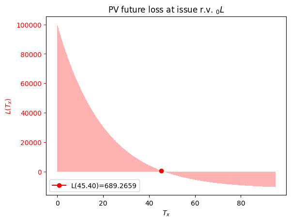
_images/bde96aa2f6ae03bb2fe72f058e1a0902b43b3a8c2b6fb8e15a401cae0660c717.png

SOA Question 6.46 : (E) 208

life = Recursion().set_interest(i=0.05)\
                  .set_IA(0.51213, x=55, t=10)\
                  .set_a(12.2758, x=55)\
                  .set_a(7.4575, x=55, t=10)
A = life.deferred_annuity(55, u=10)
IA = life.increasing_insurance(55, t=10)
a = life.temporary_annuity(55, t=10)
P = life.gross_premium(a=a, A=A, IA=IA, benefit=300)
isclose(208, P, question="Q6.46")

----- Q6.46 208: 208.12282139036515 [OK] -----

True

SOA Question 6.47 : (D) 66400

For a 10-year deferred whole life annuity-due with payments of 100,000 per year on (70), you are given:

Annual gross premiums of $G$ are payable for 10 years
First year expenses are 75% of premium
Renewal expenses for years 2 and later are 5% of premium during the premium paying period
Mortality follows the Standard Ultimate Life Table
i = 0.05

Calculate $G$ using the equivalence principle.

sult = SULT()
a = sult.temporary_annuity(70, t=10)
A = sult.deferred_annuity(70, u=10)
P = sult.gross_premium(a=a, A=A, benefit=100000, initial_premium=0.75,
                        renewal_premium=0.05)
isclose(66400, P, question="Q6.47")

----- Q6.47 66400: 66384.13293704338 [OK] -----

True

SOA Question 6.48 : (A) 3195

For a special fully discrete 5-year deferred 3-year term insurance of 100,000 on (x) you are given:

There are two premium payments, each equal to P . The first is paid at the beginning of the first year and the second is paid at the end of the 5-year deferral period
$p_x = 0.95$
$q_{x + 5} = 0.02$
$q_{x + 6} = 0.03$
$q_{x + 7} = 0.04$
$i = 0.06$

Calculate P using the equivalence principle.

x = 0
life = Recursion(depth=5).set_interest(i=0.06)\
                         .set_p(.95, x=x, t=5)\
                         .set_q(.02, x=x+5)\
                         .set_q(.03, x=x+6)\
                         .set_q(.04, x=x+7)
a = 1 + life.E_x(x, t=5)
A = life.deferred_insurance(x, u=5, t=3)
P = life.gross_premium(A=A, a=a, benefit=100000)
isclose(3195, P, question="Q6.48")

\[\begin{split}\begin{array}{llll} ~\texttt{Pure Endowment}~_{5}E_{x}~:=\\ ~~~_{5}E_{x} = ~_{5}p_{x} * v^{5}& \quad \texttt{pure endowment}\end{array}\end{split}\]

\[\begin{split}\begin{array}{llll} ~\texttt{Term Insurance}~A^1_{{x+5:\overline{3|}}}~:=\\ ~~~~~~~~~~~A^1_{{x+5:\overline{1|}}} = ~A_{{x+5:\overline{1|}}} - ~E_{x+5}& \quad \texttt{endowment insurance - pure}\\ ~~~~~A_{{x+5:\overline{3|}}} = ~A^1_{{x+5:\overline{3|}}} + ~_{3}E_{x+5}& \quad \texttt{term plus pure endowment}\\ ~~~~~~~_{3}E_{x+5} = ~_{3}p_{x+5} * v^{3}& \quad \texttt{pure endowment}\\ ~~~~~~~~~_{3}p_{x+5} = ~_{2}p_{x+6} * ~p_{x+5}& \quad \texttt{survival chain rule}\\ ~~~~~~~~~~~_{2}p_{x+6} = ~p_{x+7} * ~p_{x+6}& \quad \texttt{survival chain rule}\\ ~~~~~~~A^1_{{x+5:\overline{3|}}} = ~A_{{x+5:\overline{3|}}} - ~_{3}E_{x+5}& \quad \texttt{endowment insurance - pure}\\ ~~~~~~~~~_{3}E_{x+5} = ~E_{x+5} * ~_{2}E_{x+6}& \quad \texttt{pure endowment chain rule}\\ ~~~~~~~~~~~_{2}E_{x+6} = ~E_{x+6} * ~E_{x+7}& \quad \texttt{pure endowment chain rule}\\ ~~~~~~~~~~~~~E_{x+7} = ~p_{x+7} * v& \quad \texttt{pure endowment}\\ ~~~~~~~~~~~~~E_{x+6} = ~p_{x+6} * v& \quad \texttt{pure endowment}\\ ~~~~~~~~~~~E_{x+5} = ~p_{x+5} * v& \quad \texttt{pure endowment}\\ ~~~~~~~~~~~~~p_{x+7} = 1 - ~q_{x+7}& \quad \texttt{complement of mortality}\\ ~~~~~~~~~A^1_{{x+5:\overline{3|}}} = v * [ ~q_{x+5} * b + ~p_{x+5} * ~A^1_{{x+6:\overline{2|}}} ]& \quad \texttt{backward recursion}\\ ~~~~~~~~~~~A^1_{{x+6:\overline{2|}}} = v * [ ~q_{x+6} * b + ~p_{x+6} * ~A^1_{{x+7:\overline{1|}}} ]& \quad \texttt{backward recursion}\\ ~~~~~~~~~~~~~p_{x+6} = 1 - ~q_{x+6}& \quad \texttt{complement of mortality}\\ ~~~~~~~~~~~~~p_{x+5} = 1 - ~q_{x+5}& \quad \texttt{complement of mortality}\end{array}\end{split}\]

----- Q6.48 3195: 3195.118917658744 [OK] -----

True

SOA Question 6.49 : (C) 86

For a special whole life insurance of 100,000 on (40), you are given:

The death benefit is payable at the moment of death
Level gross premiums are payable monthly for a maximum of 20 years
Mortality follows the Standard Ultimate Life Table
$i = 0.05$
Deaths are uniformly distributed over each year of age
Initial expenses are 200
Renewal expenses are 4% of each premium including the first
Gross premiums are calculated using the equivalence principle

Calculate the monthly gross premium.

sult = SULT(udd=True)
a = UDD(m=12, life=sult).temporary_annuity(40, t=20)
A = sult.whole_life_insurance(40, discrete=False)
P = sult.gross_premium(a=a, A=A, benefit=100000, initial_policy=200,
                       renewal_premium=0.04, initial_premium=0.04) / 12
isclose(86, P, question="Q6.49")

----- Q6.49 86: 85.99177833261696 [OK] -----

True

SOA Question 6.50 : (A) -47000

On July 15, 2017, XYZ Corp buys fully discrete whole life insurance policies of 1,000 on each of its 10,000 workers, all age 35. It uses the death benefits to partially pay the premiums for the following year.

You are given:

Mortality follows the Standard Ultimate Life Table
i = 0.05
The insurance is priced using the equivalence principle

Calculate XYZ Corp’s expected net cash flow from these policies during July 2018.

life = SULT()
P = life.premium_equivalence(a=life.whole_life_annuity(35), b=1000)
a = life.deferred_annuity(35, u=1, t=1)
A = life.term_insurance(35, t=1, b=1000)
cash = (A - a * P) * 10000 / life.interest.v
isclose(-47000, cash, question="Q6.50")

----- Q6.50 -47000: -46948.218769781866 [OK] -----

True

SOA Question 6.51 : (D) 34700

life = Recursion().set_DA(0.4891, x=62, t=10)\
                   .set_A(0.0910, x=62, t=10)\
                   .set_a(12.2758, x=62)\
                   .set_a(7.4574, x=62, t=10)
IA = life.increasing_insurance(62, t=10)
A = life.deferred_annuity(62, u=10)
a = life.temporary_annuity(62, t=10)
P = life.gross_premium(a=a, A=A, IA=IA, benefit=50000)
isclose(34700, P, question="Q6.51")

\[\begin{split}\begin{array}{llll} ~\texttt{Increasing Insurance}~(IA)_{{x+62:\overline{10|}}}~:=\\ ~~~(IA)_{{x+62:\overline{10|}}} = 11 ~A^1_{{x+62:\overline{10|}}} - ~(DA)_{{x+62:\overline{10|}}}& \quad \texttt{varying insurance identity}\end{array}\end{split}\]

----- Q6.51 34700: 34687.207544453246 [OK] -----

True

SOA Question 6.52 : (D) 50.80

For a fully discrete 10-payment whole life insurance of H on (45), you are given:

Expenses payable at the beginning of each year are as follows:

Expense Type	First Year	Years 2-10	Years 11+
Per policy	100	20	10
% of Premium	105%	5%	0%

Mortality follows the Standard Ultimate Life Table
i = 0.05
The gross annual premium, calculated using the equivalence principle, is of the form $G = gH + f$, where $g$ is the premium rate per 1 of insurance and $f$ is the per policy fee

Calculate $f$.

set face value benefits to 0

sult = SULT()
a = sult.temporary_annuity(45, t=10)
other_cost = 10 * sult.deferred_annuity(45, u=10)
P = sult.gross_premium(a=a, A=0, benefit=0,    # set face value H = 0
                       initial_premium=1.05, renewal_premium=0.05,
                       initial_policy=100 + other_cost, renewal_policy=20)
isclose(50.8, P, question="Q6.52")

----- Q6.52 50.8: 50.80135534704229 [OK] -----

True

SOA Question 6.53 : (D) 720

A warranty pays 2000 at the end of the year of the first failure if a washing machine fails within three years of purchase. The warranty is purchased with a single premium, G, paid at the time of purchase of the washing machine. You are given:

10% of the washing machines that are working at the start of each year fail by the end of that year
i = 0.08
The sales commission is 35% of G
G is calculated using the equivalence principle

Calculate G.

x = 0
life = LifeTable().set_interest(i=0.08).set_table(q={x:.1, x+1:.1, x+2:.1})
A = life.term_insurance(x, t=3)
P = life.gross_premium(a=1, A=A, benefit=2000, initial_premium=0.35)
isclose(720, P, question="Q6.53")

----- Q6.53 720: 720.1646090534978 [OK] -----

True

SOA Question 6.54 : (A) 25440

For a fully discrete whole life insurance of 200,000 on (45), you are given:

Mortality follows the Standard Ultimate Life Table.
i = 0.05
The annual premium is determined using the equivalence principle.

Calculate the standard deviation of $_0L$ , the present value random variable for the loss at issue.

[A modified version of Question 12 on the Fall 2017 exam]

life = SULT()
std = math.sqrt(life.net_policy_variance(45, b=200000))
isclose(25440, std, question="Q6.54")

----- Q6.54 25440: 25441.694847703868 [OK] -----

True

7 Policy Values#

SOA Question 7.1 : (C) 11150

For a special fully discrete whole life insurance on (40), you are given:

The death benefit is 50,000 in the first 20 years and 100,000 thereafter
Level net premiums of 875 are payable for 20 years
Mortality follows the Standard Ultimate Life Table
i = 0.05

Calculate $_{10}V$ the net premium policy value at the end of year 10 for this insurance.

life = SULT()
x, n, t = 40, 20, 10
A = (life.whole_life_insurance(x+t, b=50000)
     + life.deferred_insurance(x+t, u=n-t, b=50000))
a = life.temporary_annuity(x+t, t=n-t, b=875)
L = life.gross_future_loss(A=A, a=a)
isclose(11150, L, question="Q7.1")

----- Q7.1 11150: 11152.108749338717 [OK] -----

True

SOA Question 7.2 : (C) 1152

x = 0
life = Recursion(verbose=False).set_interest(i=.1)\
                               .set_q(0.15, x=x)\
                               .set_q(0.165, x=x+1)\
                               .set_reserves(T=2, endowment=2000)

def fun(P):  # solve P s.t. V is equal backwards and forwards
    policy = dict(t=1, premium=P, benefit=lambda t: 2000, reserve_benefit=True)
    return life.t_V_backward(x, **policy) - life.t_V_forward(x, **policy)
P = life.solve(fun, target=0, grid=[1070, 1230])
isclose(1152, P, question="Q7.2")

----- Q7.2 1152: 1151.5151515151515 [OK] -----

True

SOA Question 7.3 : (E) 730

x = 0  # x=0 is (90) and interpret every 3 months as t=1 year
life = LifeTable().set_interest(i=0.08/4)\
                  .set_table(l={0:1000, 1:898, 2:800, 3:706})\
                  .set_reserves(T=8, V={3: 753.72})
V = life.t_V_backward(x=0, t=2, premium=60*0.9, benefit=lambda t: 1000)
V = life.set_reserves(V={2: V})\
        .t_V_backward(x=0, t=1, premium=0, benefit=lambda t: 1000)
isclose(730, V, question="Q7.3")

----- Q7.3 730: 729.998398765594 [OK] -----

True

SOA Question 7.4 : (B) -74

For a special fully discrete whole life insurance on (40), you are given:

The death benefit is 1000 during the first 11 years and 5000 thereafter
Expenses, payable at the beginning of the year, are 100 in year 1 and 10 in years 2 and later
$\pi$ is the level annual premium, determined using the equivalence principle
$G = 1.02 \times \pi$ is the level annual gross premium
Mortality follows the Standard Ultimate Life Table
i = 0.05
$_{11}E_{40} = 0.57949$

Calculate the gross premium policy value at the end of year 1 for this insurance.

hints:

split benefits into two policies

life = SULT()
P = life.gross_premium(a=life.whole_life_annuity(40),
                       A=life.whole_life_insurance(40),
                       initial_policy=100, renewal_policy=10,
                       benefit=1000)
P += life.gross_premium(a=life.whole_life_annuity(40),
                        A=life.deferred_insurance(40, u=11),
                        benefit=4000)   # for deferred portion
contract = Contract(benefit=1000, premium=1.02*P,
                    renewal_policy=10, initial_policy=100)
V = life.gross_policy_value(x=40, t=1, contract=contract)
contract = Contract(benefit=4000, premium=0)
A = life.deferred_insurance(41, u=10)
V += life.gross_future_loss(A=A, a=0, contract=contract)   # for deferred portion
isclose(-74, V, question="Q7.4")

----- Q7.4 -74: -73.94215569524829 [OK] -----

True

SOA Question 7.5 : (E) 1900

For a fully discrete whole life insurance of 10,000 on (x), you are given:

Deaths are uniformly distributed over each year of age
The net premium is 647.46
The net premium policy value at the end of year 4 is 1405.08
$q_{x+4}$ = 0.04561
i = 0.03

Calculate the net premium policy value at the end of 4.5 years.

x = 0
life = Recursion(udd=True).set_interest(i=0.03)\
                          .set_q(0.04561, x=x+4)\
                          .set_reserves(T=3, V={4: 1405.08})
V = life.r_V_forward(x, s=4, r=0.5, benefit=10000, premium=647.46)
isclose(1900, V, question="Q7.5")

----- Q7.5 1900: 1901.766021537228 [OK] -----

True

Answer 7.6: (E) -25.4

life = SULT()
P = life.net_premium(45, b=2000)
contract = Contract(benefit=2000, initial_premium=.25, renewal_premium=.05,
                    initial_policy=2*1.5 + 30, renewal_policy=2*.5 + 10)
G = life.gross_premium(a=life.whole_life_annuity(45), **contract.premium_terms)
gross = life.gross_policy_value(45, t=10, contract=contract.set_contract(premium=G))
net = life.net_policy_value(45, t=10, b=2000)
V = gross - net
isclose(-25.4, V, question="Q7.6")

----- Q7.6 -25.4: -25.44920289521201 [OK] -----

True

SOA Question 7.7 : (D) 1110

For a whole life insurance of 10,000 on (x), you are given:

Death benefits are payable at the end of the year of death
A premium of 30 is payable at the start of each month
Commissions are 5% of each premium
Expenses of 100 are payable at the start of each year
$i = 0.05$
$1000 A_{x+10} = 400$
$_{10} V$ is the gross premium policy value at the end of year 10 for this insurance

Calculate $_{10} V$ using the two-term Woolhouse formula for annuities.

x = 0
life = Recursion().set_interest(i=0.05).set_A(0.4, x=x+10)
a = Woolhouse(m=12, life=life).whole_life_annuity(x+10)
contract = Contract(premium=0, benefit=10000, renewal_policy=100)
V = life.gross_future_loss(A=0.4, contract=contract.renewals())
contract = Contract(premium=30*12, renewal_premium=0.05)
V += life.gross_future_loss(a=a, contract=contract.renewals())
isclose(1110, V, question="Q7.7")

\[\begin{split}\begin{array}{llll} ~\texttt{Whole Life Annuity}~\ddot{a}_{{x+10}}~:=\\ ~~~\ddot{a}_{{x+10}} = [1 - ~A_{{x+10}} ] / d& \quad \texttt{insurance twin}\end{array}\end{split}\]

----- Q7.7 1110: 1107.9718253968258 [OK] -----

True

SOA Question 7.8 : (C) 29.85

sult = SULT()
x = 70
q = {x: [sult.q_x(x+k)*(.7 + .1*k) for k in range(3)] + [sult.q_x(x+3)]}
life = Recursion().set_interest(i=.05)\
                  .set_q(sult.q_x(70)*.7, x=x)\
                  .set_reserves(T=3)
V = life.t_V(x=70, t=1, premium=35.168, benefit=lambda t: 1000)
isclose(29.85, V, question="Q7.8")

\[\begin{split}\begin{array}{llll} ~\texttt{Survival}~p_{x+70}~:=\\ ~~~p_{x+70} = 1 - ~q_{x+70}& \quad \texttt{complement of mortality}\end{array}\end{split}\]

----- Q7.8 29.85: 29.85469179271202 [OK] -----

True

SOA Question 7.9 : (A) 38100

For a semi-continuous 20-year endowment insurance of 100,000 on (45), you are given:

Net premiums of 253 are payable monthly
Mortality follows the Standard Ultimate Life Table
Deaths are uniformly distributed over each year of age
$i = 0.05$

Calculate $_{10}V$, the net premium policy value at the end of year 10 for this insurance.

sult = SULT(udd=True)
x, n, t = 45, 20, 10
a = UDD(m=12, life=sult).temporary_annuity(x=x+10, t=n-t)
A = UDD(m=0, life=sult).endowment_insurance(x=x+10, t=n-t)
contract = Contract(premium=253*12, endowment=100000, benefit=100000)
V = sult.gross_future_loss(A=A, a=a, contract=contract)
isclose(38100, V, question="Q7.9")

----- Q7.9 38100: 38099.62176709246 [OK] -----

True

SOA Question 7.10 : (C) -970

For a fully discrete whole life insurance of 100,000 on (45), you are given:

Mortality follows the Standard Ultimate Life Table
i = 0.05
Commission expenses are 60% of the first year’s gross premium and 2% of renewal gross premiums
Administrative expenses are 500 in the first year and 50 in each renewal year
All expenses are payable at the start of the year
The gross premium, calculated using the equivalence principle, is 977.60

Calculate $_5V^e$, the expense reserve at the end of year 5 for this insurance.

life = SULT()
G = 977.6
P = life.net_premium(45, b=100000)
contract = Contract(benefit=0, premium=G-P, renewal_policy=.02*G + 50)
V = life.gross_policy_value(45, t=5, contract=contract)
isclose(-970, V, question="Q7.10")

----- Q7.10 -970: -971.8909301877864 [OK] -----

True

SOA Question 7.11 : (B) 1460

life = Recursion().set_interest(i=0.05).set_a(13.4205, x=55)
contract = Contract(benefit=10000)
def fun(P):
    return life.L_from_t(t=10, contract=contract.set_contract(premium=P))
P = life.solve(fun, target=4450, grid=400)
V = life.gross_policy_value(45, t=10, contract=contract.set_contract(premium=P))
isclose(1460, V, question="Q7.11")

\[\begin{split}\begin{array}{llll} ~\texttt{Whole Life Insurance}~A_{{x+55}}~:=\\ ~~~\ddot{a}_{{x+55}} = [ 1 - ~A_{{x+55}} ] / d& \quad \texttt{annuity twin}\end{array}\end{split}\]

----- Q7.11 1460: 1459.9818035330204 [OK] -----

True

SOA Question 7.12 : (E) 4.09

For a special fully discrete 25-year endowment insurance on (44), you are given:

The death benefit is ( 26−k ) for death in year ,k for k = 1,2,3,…,25
The endowment benefit in year 25 is 1
Net premiums are level
$q_{55}$= 0.15
i = 0.04
$_{11}V$ the net premium policy value at the end of year 11, is 5.00
$_{24}V$ the net premium policy value at the end of year 24, is 0.60

Calculate $_{12}V$ the net premium policy value at end of year 12.

benefit = lambda k: 26 - k
x = 44
life = Recursion().set_interest(i=0.04)\
                  .set_q(0.15, x=55)\
                  .set_reserves(T=25, endowment=1, V={11: 5.})
def fun(P):  # solve for net premium, from final year recursion
    return life.t_V(x=x, t=24, premium=P, benefit=benefit)
P = life.solve(fun, target=0.6, grid=0.5)    # solved net premium
V = life.t_V(x, t=12, premium=P, benefit=benefit)  # recursion formula
isclose(4.09, V, question="Q7.12")

\[\begin{split}\begin{array}{llll} ~\texttt{Survival}~p_{x+55}~:=\\ ~~~p_{x+55} = 1 - ~q_{x+55}& \quad \texttt{complement of mortality}\end{array}\end{split}\]

----- Q7.12 4.09: 4.089411764705883 [OK] -----

True

SOA Question 7.13 : (A) 180

life = SULT()
V = life.FPT_policy_value(40, t=10, n=30, endowment=1000, b=1000)
isclose(180, V, question="Q7.13")

----- Q7.13 180: 180.10717859040767 [OK] -----

True

SOA Question 7.14 : (A) 2200

For a fully discrete whole life insurance of 100,000 on (45), you are given:

The gross premium policy value at duration 5 is 5500 and at duration 6 is 7100
$q_{50}$ = 0.009
i = 0.05
Renewal expenses at the start of each year are 50 plus 4% of the gross premium.
Claim expenses are 200.

Calculate the gross premium.

x = 45
life = Recursion(verbose=False).set_interest(i=0.05)\
                               .set_q(0.009, x=50)\
                               .set_reserves(T=10, V={5: 5500})
def fun(P):  # solve for net premium,
    return life.t_V(x=x, t=6, premium=P*0.96 - 50, benefit=lambda t: 100000+200)
P = life.solve(fun, target=7100, grid=[2200, 2400])
isclose(2200, P, question="Q7.14")

----- Q7.14 2200: 2197.8174603174602 [OK] -----

True

SOA Question 7.15 : (E) 50.91

For a fully discrete whole life insurance of 100 on (x), you are given:

$q_{x+ 15} = 0.10$
Deaths are uniformly distributed over each year of age
i = 0.05
$_tV$ denotes the net premium policy value at time t
$_{16}V$ = 49.78

Calculate 15.6.

x = 0
V = Recursion(udd=True).set_interest(i=0.05)\
                       .set_q(0.1, x=x+15)\
                       .set_reserves(T=3, V={16: 49.78})\
                       .r_V_backward(x, s=15, r=0.6, benefit=100)
isclose(50.91, V, question="Q7.15")

----- Q7.15 50.91: 50.91362826922369 [OK] -----

True

SOA Question 7.16 : (D) 380

life = SelectLife().set_interest(v=.95)\
                   .set_table(A={86: [683/1000]},
                              q={80+k: [.01*(k+1)] for k in range(6)})
x, t, n = 80, 3, 5
A = life.whole_life_insurance(x+t)
a = life.temporary_annuity(x+t, t=n-t)
V = life.gross_future_loss(A=A, a=a, contract=Contract(benefit=1000, premium=130))
isclose(380, V, question="Q7.16")

----- Q7.16 380: 381.6876905200001 [OK] -----

True

SOA Question 7.17 : (D) 1.018

x = 0
life = Recursion().set_interest(v=math.sqrt(0.90703))\
                  .set_q(0.02067, x=x+10)\
                  .set_A(0.52536, x=x+11)\
                  .set_A(0.30783, x=x+11, moment=2)
A1 = life.whole_life_insurance(x+10)
A2 = life.whole_life_insurance(x+10, moment=2)
ratio = (life.insurance_variance(A2=A2, A1=A1)
         / life.insurance_variance(A2=0.30783, A1=0.52536))
isclose(1.018, ratio, question="Q7.17")

\[\begin{split}\begin{array}{llll} ~\texttt{Whole Life Insurance}~A_{{x+10}}~:=\\ ~~~A_{{x+10}} = v * [ ~q_{x+10} * b + ~p_{x+10} * ~A_{{x+11}} ]& \quad \texttt{backward recursion}\\ ~~~~~p_{x+10} = 1 - ~q_{x+10}& \quad \texttt{complement of mortality}\end{array}\end{split}\]

\[\begin{split}\begin{array}{llll} ~\texttt{Whole Life Insurance}~^2A_{{x+10}}~:=\\ ~~~^2A_{{x+10}} = v^{2} * [ ~q_{x+10} * b^{2} + ~p_{x+10} * ~^2A_{{x+11}} ]& \quad \texttt{backward recursion}\\ ~~~~~p_{x+10} = 1 - ~q_{x+10}& \quad \texttt{complement of mortality}\end{array}\end{split}\]

----- Q7.17 1.018: 1.0182465434445054 [OK] -----

True

SOA Question 7.18 : (A) 17.1

For a fully discrete whole life insurance of 1 on (x), you are given:

The net premium policy value at the end of the first year is 0.012
$q_x$ = 0.009
i = 0.04

Calculate $\ddot{a}_x$

x = 10
life = Recursion(verbose=False).set_interest(i=0.04).set_q(0.009, x=x)
def fun(a):
    return life.set_a(a, x=x).net_policy_value(x, t=1)
a = life.solve(fun, target=0.012, grid=[17.1, 19.1])
isclose(17.1, a, question="Q7.18")

----- Q7.18 17.1: 17.07941929974388 [OK] -----

True

SOA Question 7.19 : (D) 720

For a fully discrete whole life insurance of 100,000 on (40) you are given:

Expenses incurred at the beginning of the first year are 300 plus 50% of the first year premium
Renewal expenses, incurred at the beginning of the year, are 10% of each of the renewal premiums
Mortality follows the Standard Ultimate Life Table
i = 0.05
Gross premiums are calculated using the equivalence principle

Calculate the gross premium policy value for this insurance immediately after the second premium and associated renewal expenses are paid.

life = SULT()
contract = Contract(benefit=100000,
                    initial_policy=300,
                    initial_premium=.5,
                    renewal_premium=.1)
P = life.gross_premium(A=life.whole_life_insurance(40), **contract.premium_terms)
A = life.whole_life_insurance(41)
a = life.immediate_annuity(41)   # after premium and expenses are paid
V = life.gross_future_loss(A=A,
                           a=a,
                           contract=contract.set_contract(premium=P).renewals())
isclose(720, V, question="Q7.19")

----- Q7.19 720: 722.7510208759013 [OK] -----

True

SOA Question 7.20 : (E) -277.23

For a fully discrete whole life insurance of 1000 on (35), you are given:

First year expenses are 30% of the gross premium plus 300
Renewal expenses are 4% of the gross premium plus 30
All expenses are incurred at the beginning of the policy year
Gross premiums are calculated using the equivalence principle
The gross premium policy value at the end of the first policy year is R
Using the Full Preliminary Term Method, the modified reserve at the end of the first policy year is S
Mortality follows the Standard Ultimate Life Table
i = 0.05

Calculate R−S .

life = SULT()
S = life.FPT_policy_value(35, t=1, b=1000)  # is 0 for FPT at t=0,1
contract = Contract(benefit=1000,
                    initial_premium=.3,
                    initial_policy=300,
                    renewal_premium=.04,
                    renewal_policy=30)
G = life.gross_premium(A=life.whole_life_insurance(35), **contract.premium_terms)
R = life.gross_policy_value(35, t=1, contract=contract.set_contract(premium=G))
isclose(-277.23, R - S, question="Q7.20")

----- Q7.20 -277.23: -277.1930332392921 [OK] -----

True

SOA Question 7.21 : (D) 11866

life = SULT()
x, t, u = 55, 9, 10
P = life.gross_premium(IA=0.14743,
                       a=life.temporary_annuity(x, t=u),
                       A=life.deferred_annuity(x, u=u),
                       benefit=1000)
contract = Contract(initial_policy=life.term_insurance(x+t, t=1, b=10*P),
                    premium=P,
                    benefit=1000)
a = life.temporary_annuity(x+t, t=u-t)
A = life.deferred_annuity(x+t, u=u-t)
V = life.gross_future_loss(A=A, a=a, contract=contract)
isclose(11866, V, question="Q7.21")

----- Q7.21 11866: 11866.301581004533 [OK] -----

True

SOA Question 7.22 : (C) 46.24

life = PolicyValues().set_interest(i=0.06)
contract = Contract(benefit=8, premium=1.250)
def fun(A2):
    return life.gross_variance_loss(A1=0, A2=A2, contract=contract)
A2 = life.solve(fun, target=20.55, grid=20.55/8**2)
contract = Contract(benefit=12, premium=1.875)
var = life.gross_variance_loss(A1=0, A2=A2, contract=contract)
isclose(46.2, var, question="Q7.22")

----- Q7.22 46.2: 46.2375 [OK] -----

True

SOA Question 7.23 : (D) 233

life = Recursion().set_interest(i=0.04).set_p(0.995, x=25)
A = life.term_insurance(25, t=1, b=10000)
def fun(beta):  # value of premiums in first 20 years must be equal
    return beta * 11.087 + (A - beta)
beta = life.solve(fun, target=216 * 11.087, grid=[140, 260])
isclose(233, beta, question="Q7.23")

\[\begin{split}\begin{array}{llll} ~\texttt{Term Insurance}~A^1_{{x+25:\overline{1|}}}* 10000~:=\\ ~~~A^1_{{x+25:\overline{1|}}} = ~A_{{x+25:\overline{1|}}} - ~E_{x+25}& \quad \texttt{endowment insurance - pure}\\ ~~~~~E_{x+25} = ~p_{x+25} * v& \quad \texttt{pure endowment}\end{array}\end{split}\]

----- Q7.23 233: 232.64747466274179 [OK] -----

True

SOA Question 7.24 : (C) 680

For a fully discrete whole life insurance policy of 1,000,000 on (50), you are given:

The annual gross premium, calculated using the equivalence principle, is 11,800
Mortality follows the Standard Ultimate Life Table
i = 0.05

Calculate the expense loading, P for this policy.

life = SULT()
P = life.premium_equivalence(A=life.whole_life_insurance(50), b=1000000)
isclose(680, 11800 - P, question="Q7.24")

----- Q7.24 680: 680.2918236453952 [OK] -----

True

SOA Question 7.25 : (B) 3947.37

life = SelectLife().set_interest(i=.04)\
                   .set_table(A={55: [.23, .24, .25],
                                 56: [.25, .26, .27],
                                 57: [.27, .28, .29],
                                 58: [.20, .30, .31]})
V = life.FPT_policy_value(55, t=3, b=100000)
isclose(3950, V, question="Q7.25")

----- Q7.25 3950: 3947.3684210526353 [OK] -----

True

SOA Question 7.26 : (D) 28540

backward = forward reserve recursion

x = 0
life = Recursion(verbose=False).set_interest(i=.05)\
                               .set_p(0.85, x=x)\
                               .set_p(0.85, x=x+1)\
                               .set_reserves(T=2, endowment=50000)
def benefit(k): return k * 25000
def fun(P):  # solve P s.t. V is equal backwards and forwards
    policy = dict(t=1, premium=P, benefit=benefit, reserve_benefit=True)
    return life.t_V_backward(x, **policy) - life.t_V_forward(x, **policy)
P = life.solve(fun, target=0, grid=[27650, 28730])
isclose(28540, P, question="Q7.26")

----- Q7.26 28540: 28542.392566782808 [OK] -----

True

SOA Question 7.27 : (B) 213

x = 0
life = Recursion(verbose=False).set_interest(i=0.03)\
                               .set_q(0.008, x=x)\
                               .set_reserves(V={0: 0})
def fun(G):  # Solve gross premium from expense reserves equation
    return life.t_V(x=x, t=1, premium=G - 187, benefit=lambda t: 0,
                    per_policy=10 + 0.25*G)
G = life.solve(fun, target=-38.70, grid=[200, 252])
isclose(213, G, question="Q7.27")

----- Q7.27 213: 212.970355987055 [OK] -----

True

SOA Question 7.28 : (D) 24.3

life = SULT()
PW = life.net_premium(65, b=1000)   # 20_V=0 => P+W is net premium for A_65
P = life.net_premium(45, t=20, b=1000)  # => P is net premium for A_45:20
isclose(24.3, PW - P, question="Q7.28")

----- Q7.28 24.3: 24.334725400123986 [OK] -----

True

SOA Question 7.29 : (E) 2270

For a fully discrete whole life insurance of B on (x), you are given:

Expenses, incurred at the beginning of each year, equal 30 in the first year and 5 in subsequent years
The net premium policy value at the end of year 10 is 2290
Gross premiums are calculated using the equivalence principle
i = 0.04
$\ddot{a}_x$ = 14.8
$\ddot{a}_{x+10}$ = 11.4

Calculate $_{10}V^{g}$, the gross premium policy value at the end of year 10.

x = 0
life = Recursion(verbose=False).set_interest(i=0.04)\
                               .set_a(14.8, x=x)\
                               .set_a(11.4, x=x+10)
def fun(B):
    return life.net_policy_value(x, t=10, b=B)
B = life.solve(fun, target=2290, grid=2290*10)  # Solve benefit B given net 10_V
contract = Contract(initial_policy=30, renewal_policy=5, benefit=B)
G = life.gross_premium(a=life.whole_life_annuity(x), **contract.premium_terms)
V = life.gross_policy_value(x, t=10, contract=contract.set_contract(premium=G))
isclose(2270, V, question="Q7.29")

----- Q7.29 2270: 2270.743243243244 [OK] -----

True

SOA Question 7.30 : (E) 9035

Ten years ago J, then age 25, purchased a fully discrete 10-payment whole life policy of 10,000.

All actuarial calculations for this policy were based on the following:

Mortality follows the Standard Ultimate Life Table
i = 0.05
The equivalence principle

In addition:

$L_{10}$ is the present value of future losses random variable at time 10
At the end of policy year 10, the interest rate used to calculate $L_{10}$ is changed to 0%

Calculate the increase in $E[L_{10}]$ that results from this change.

b = 10000  # premiums=0 after t=10
L = SULT().set_interest(i=0.05).whole_life_insurance(x=35, b=b)
V = SULT().set_interest(i=0).whole_life_insurance(x=35, b=b)
isclose(9035, V - L, question="Q7.30")

----- Q7.30 9035: 9034.654127845053 [OK] -----

True

SOA Question 7.31 : (E) 0.310

For a fully discrete 3-year endowment insurance of 1000 on (x), you are given:

Expenses, payable at the beginning of the year, are:

Year(s)	Percent of Premium	Per Policy
1	20%	15
2 and 3	8%	5

The expense reserve at the end of year 2 is –23.64
The gross annual premium calculated using the equivalence principle is G = 368.
$G = 1000 P_{x:\overline{3|}} + P^e$ , where $P^e$ is the expense loading

Calculate $P_{x:\overline{3|}}$ .

x = 0
life = Reserves().set_reserves(T=3)
G = 368.05
def fun(P):  # solve net premium expense reserve equation
    return life.t_V(x, t=2, premium=G-P, benefit=lambda t:0, per_policy=5+0.08*G)
P = life.solve(fun, target=-23.64, grid=[.29, .31]) / 1000
isclose(0.310, P, question="Q7.31")

----- Q7.31 0.31: 0.309966 [OK] -----

True

SOA Question 7.32 : (B) 1.4

For two fully continuous whole life insurance policies on (x), you are given:

	Death Benefit	Annual Premium Rate	Variance of the PV of Future Loss at t
Policy A	1	0.10	0.455
Policy B	2	0.16	-

$\delta= 0.06$

Calculate the variance of the present value of future loss at $t$ for Policy B.

life = PolicyValues().set_interest(i=0.06)
contract = Contract(benefit=1, premium=0.1)
def fun(A2):
    return life.gross_variance_loss(A1=0, A2=A2, contract=contract)
A2 = life.solve(fun, target=0.455, grid=0.455)
contract = Contract(benefit=2, premium=0.16)
var = life.gross_variance_loss(A1=0, A2=A2, contract=contract)
isclose(1.39, var, question="Q7.32")

----- Q7.32 1.39: 1.3848168384380901 [OK] -----

True

Final Score

from datetime import datetime
print(datetime.now())
print(isclose)

2026-04-22 11:47:25.120549
Elapsed: 11.5 secs
Passed:  136/136

\(x\)	\(l_{[x]}\)	\(d_{[x]}\)	\(l_{x+1}\)	\(x + 1\)
65	1000	40	−	66
66	955	45	−	67

FAM-L Exam Solutions and Hints

Contents

FAM-L Exam Solutions and Hints#

1 Tables#

2 Survival models#

3 Life tables and selection#

4 Insurance benefits#

5 Annuities#

6 Premium Calculation#

7 Policy Values#